Varenicline PK and exposure-response in adolescent smokers (Fediuk 2021)

Model and source

Fediuk 2021 pooled two phase 1 PK studies and one phase 4 efficacy and safety study of varenicline in adolescent smokers. It fitted a population PK model and then two logistic exposure-response (ER) models on the phase 4 subjects, driven by the individual steady-state daily exposure AUC(0-24) from the PK model. The three analyses were fitted separately (NONMEM 7.3; FOCE-I for PK, Laplacian likelihood for ER), so they are packaged as three model files:

Model	Endpoint	n
Fediuk_2021_varenicline	Plasma varenicline, one-compartment popPK	218
Fediuk_2021_varenicline_nausea	Nausea or vomiting incidence over the 12-week treatment period (final model)	238
Fediuk_2021_varenicline_car_w9_12	Continuous abstinence rate, weeks 9-12 (base model, digitized)	238

• Citation: Fediuk DJ, Sweeney K, Sahasrabudhe V, McRae T, Byon W. Population pharmacokinetics and exposure-response analyses of varenicline in adolescent smokers. CPT Pharmacometrics Syst Pharmacol. 2021;10(7):769-781. doi:10.1002/psp4.12645
• Article: https://doi.org/10.1002/psp4.12645 (open access, PMC8302239)
• Supplement: Text S1 (popPK control stream), Text S2 (nausea/vomiting control stream), Table S1 (base-model building) and Table S2 (nausea/vomiting estimates), all from the article’s Supporting Information.
• Adult comparator already in the library: Ravva_2009_varenicline (popPK) and Ravva_2010_varenicline_nausea (adult ER, same model shape).

mod_pk <- readModelDb("Fediuk_2021_varenicline")
mod_nv <- readModelDb("Fediuk_2021_varenicline_nausea")
mod_car <- readModelDb("Fediuk_2021_varenicline_car_w9_12")

Population

The popPK analysis used 1,097 plasma concentrations from 218 varenicline-treated adolescents (Fediuk 2021 Table 2): 22 from a single-dose phase 1 study (0.5 or 1 mg; 86% Black), 57 from a 14-day multiple-dose phase 1 study and 139 from the 12-week phase 4 study. Median age was 16 years (range 12-20), median body weight 62.1 kg (35.0-121), 37.6% were female, and the race mix was 65.1% White, 14.2% Black, 11.9% Asian and 8.7% other. About 99% had normal renal function. Doses were weight-banded: 0.5 mg q.d. or 0.5 mg b.i.d. for body weight up to 55 kg, and 0.5 mg b.i.d. or 1 mg b.i.d. above 55 kg.

The ER analyses used the 238 phase 4 subjects with one observation each: 99 on placebo (AUC24 = 0) and 139 on varenicline with at least one measurable concentration. They were 34% female, 73.9% White, 6.7% Black and 19.3% Asian/other, and 81% smoked their first cigarette within 30 minutes of waking.

The same information is available programmatically via each model’s population metadata (e.g. readModelDb("Fediuk_2021_varenicline")()$population).

Source trace

Every ini() value carries an in-file comment naming its source. They are collected here.

Population PK (Fediuk_2021_varenicline)

Parameter	Value	Source location
lcl (CL/F, L/h)	log(12.5)	Table 3; Text S1 THETA(1)
lvc (V/F, L)	log(231)	Table 3; Text S1 THETA(2)
lka (1/h)	log(0.860)	Table 3; Text S1 THETA(3)
e_wt_cl, e_wt_vc	0.567, 0.872	Table 3 ‘Body weight’ rows; Text S1 THETA(4), THETA(5)
e_race_black_cl, e_race_other_cl, e_sexf_cl	1.01, 1.12, 0.850	Table 3 CL/F rows; Text S1 THETA(6)-THETA(8)
e_race_black_vc, e_race_other_vc, e_sexf_vc	0.757, 0.854, 0.861	Table 3 V/F rows; Text S1 THETA(9)-THETA(11)
etalcl + etalvc + etalka block	0.102; -0.00162, 0.0182; -0.0582, 0.0307, 0.174	Table 3 omega2 and COV rows
propSdPh1, addSdPh1	0.291, 0.240 ng/mL	Table 3 sigma2 0.0847, 0.0577 (0.240 ng/mL); Results ‘29.1%’
propSdPh4, addSdPh4	0.432, 0.580 ng/mL	Table 3 sigma2 0.187, 0.336 (0.580 ng/mL); Results ‘43.2%’
Covariate equations	power on WT/70; theta^indicator	Methods equations; Text S1 $PK
One-compartment first-order absorption	n/a	Methods; Text S1 ADVAN2 TRANS2
Cc = 1000 * central / vc	n/a	Text S1 S2 = V/1000 (mg dose, ng/mL)
Study-stratum residual switch	n/a	Text S1 $ERROR IF(PROT.EQ.1073) IND = 1

Nausea or vomiting (Fediuk_2021_varenicline_nausea)

Parameter	Value	Source location
base_logit	-30.9	Table S2 theta1; Text S2 THETA(1)
e_auc_varen_base_logit (per ng*h/mL)	0.00911	Table S2 theta2
e_smoke_ttfc_31_60_base_logit, _6_30_, _le5_	0.0750, 0.0773, 0.0779	Table S2 theta3-theta5
e_age_base_logit (on AGE/16)	-0.296	Table S2 theta6
e_sexf_base_logit	0.554	Table S2 theta7
e_race_black_base_logit, e_race_other_base_logit	0.870, 0.966	Table S2 theta8, theta9
etabase_logit	fixed(0)	Text S2 $OMEGA 0 FIX
Logit equation	covariates multiply the intercept, AUC additive	Methods equation; Text S2 LGT
addSd	fixed(0.001)	Not paper-derived (placeholder; see Assumptions)

Continuous abstinence weeks 9-12 (Fediuk_2021_varenicline_car_w9_12)

Parameter	Value	Source location
base_logit	-1.42	Digitized from the Figure 3a ‘Model predicted’ line (not printed)
e_auc_varen_base_logit (per ng*h/mL)	0.00211	Digitized from Figure 3a (not printed; Results give only p = 0.303)
addSd	fixed(0.001)	Not paper-derived (placeholder; see Assumptions)

Population PK

Covariate effects on AUC24 (Figure 2)

Figure 2 prints the ratio of typical AUC24 to that of the 70 kg White male reference. Because AUC24 = daily dose / (CL/F), each ratio is the inverse of the typical CL/F ratio, so the model must reproduce all five printed values to the two printed decimals.

ref_cov <- data.frame(WT = 70, SEXF = 0, RACE_BLACK = 0, RACE_OTHER = 0)
fig2 <- tibble::tribble(
  ~label,         ~WT, ~SEXF, ~RACE_BLACK, ~RACE_OTHER, ~published,
  "Weight 60 kg",  60,     0,           0,           0,       1.09,
  "Weight 80 kg",  80,     0,           0,           0,       0.93,
  "Race (black)",  70,     0,           1,           0,       0.99,
  "Race (other)",  70,     0,           0,           1,       0.89,
  "Sex (female)",  70,     1,           0,           0,       1.18
)
typical_cl <- function(cov) {
  ev <- dplyr::bind_cols(
    data.frame(id = seq_len(nrow(cov)), time = 0, evid = 0, amt = 0,
               cmt = "central", STUDY_PHASE4 = 0),
    cov
  )
  rxode2::rxSolve(rxode2::zeroRe(mod_pk), ev, returnType = "data.frame")$cl
}
cl_ref <- typical_cl(ref_cov)
#> ℹ parameter labels from comments will be replaced by 'label()'
#> Warning: No sigma parameters in the model
#> ℹ omega/sigma items treated as zero: 'etalcl', 'etalvc', 'etalka'
fig2$model <- cl_ref / typical_cl(fig2[, c("WT", "SEXF", "RACE_BLACK", "RACE_OTHER")])
#> ℹ parameter labels from comments will be replaced by 'label()'
#> Warning: No sigma parameters in the model
#> ℹ omega/sigma items treated as zero: 'etalcl', 'etalvc', 'etalka'
#> Warning: multi-subject simulation without without 'omega'
stopifnot(nrow(fig2) == 5, abs(cl_ref - 12.5) < 1e-6)
# Deterministic: the unrounded ratio must round to the printed value.
stopifnot(all(abs(fig2$model - fig2$published) <= 0.005 + 1e-9))

fig2 |>
  dplyr::select(label, published, model) |>
  dplyr::mutate(model = signif(model, 4)) |>
  dplyr::rename("Covariate" = label, "Figure 2 ratio" = published,
                "Model ratio" = model) |>
  knitr::kable(caption = "Typical AUC24 relative to a 70 kg White male.")

Typical AUC24 relative to a 70 kg White male.

Covariate	Figure 2 ratio	Model ratio
Weight 60 kg	1.09	1.0910
Weight 80 kg	0.93	0.9271
Race (black)	0.99	0.9901
Race (other)	0.89	0.8929
Sex (female)	1.18	1.1760

Comparison with adults (Discussion)

The Discussion states that the adolescent CL/F and V/F are about 20% higher and 31% lower than in adults (Ravva 2009), and that the higher CL/F means an about 17% lower AUC24. The adult model is in the library, so the arithmetic can be checked directly from both parameter sets.

th_ad <- rxode2::rxode2(readModelDb("Fediuk_2021_varenicline"))$theta
#> ℹ parameter labels from comments will be replaced by 'label()'
th_adult <- rxode2::rxode2(readModelDb("Ravva_2009_varenicline"))$theta
cl_pct <- 100 * (exp(th_ad[["lcl"]]) / exp(th_adult[["lcl"]]) - 1)
v_pct <- 100 * (1 - exp(th_ad[["lvc"]]) / exp(th_adult[["lvc"]]))
auc_pct <- 100 * (1 - exp(th_adult[["lcl"]]) / exp(th_ad[["lcl"]]))
adult_tab <- data.frame(
  Claim = c("CL/F higher than adults (%)", "V/F lower than adults (%)",
            "AUC24 lower than adults (%)"),
  Paper = c(20, 31, 17),
  Model = round(c(cl_pct, v_pct, auc_pct), 1)
)
stopifnot(all(abs(adult_tab$Model - adult_tab$Paper) < 1))
knitr::kable(adult_tab)

Claim	Paper	Model
CL/F higher than adults (%)	20	20.2
V/F lower than adults (%)	31	31.5
AUC24 lower than adults (%)	17	16.8

The typical adolescent half-life is 12.8 h (ln 2 x V/F / CL/F), shorter than the ~24 h reported in adults, which the authors attribute to the smaller apparent volume.

Virtual cohorts

Each Figure 1 panel is simulated with 100 subjects. Body weight is drawn from a normal distribution matching the pooled popPK cohort (mean 63.9, SD 13.5 kg, Table 2) and redrawn until it falls in the panel’s weight band (low body weight at most 55 kg, high body weight above 55 kg); the band is a definition, so weights are never clamped. Sex and race follow the Table 2 proportions of the contributing studies.

set.seed(20210629)
draw_wt <- function(n, lo, hi) {
  out <- numeric(0)
  while (length(out) < n) {
    w <- stats::rnorm(4 * n, 63.9, 13.5)
    out <- c(out, w[w > lo & w <= hi])
  }
  out[seq_len(n)]
}
draw_race <- function(n, p_black, p_other) {
  u <- stats::runif(n)
  data.frame(RACE_BLACK = as.integer(u < p_black),
             RACE_OTHER = as.integer(u >= p_black & u < p_black + p_other))
}
n_arm <- 100L
arms <- tibble::tribble(
  ~arm,                                ~dose, ~bid,  ~lo,  ~hi, ~single, ~p_f,  ~p_black, ~p_other,
  "0.5 mg single dose",                  0.5, FALSE, 35,   121,  TRUE,   0.409, 0.864,    0,
  "1 mg single dose",                    1.0, FALSE, 35,   121,  TRUE,   0.409, 0.864,    0,
  "0.5 mg q.d. low body weight",         0.5, FALSE, 35,   55,   FALSE,  0.376, 0.142,    0.206,
  "0.5 mg b.i.d. high body weight",      0.5, TRUE,  55,   121,  FALSE,  0.376, 0.142,    0.206,
  "0.5 mg b.i.d. low body weight",       0.5, TRUE,  35,   55,   FALSE,  0.376, 0.142,    0.206,
  "1 mg b.i.d. high body weight",        1.0, TRUE,  55,   121,  FALSE,  0.376, 0.142,    0.206
)
make_arm <- function(k) {
  a <- arms[k, ]
  subj <- data.frame(
    id = (k - 1L) * n_arm + seq_len(n_arm),
    WT = draw_wt(n_arm, a$lo, a$hi),
    SEXF = stats::rbinom(n_arm, 1, a$p_f),
    STUDY_PHASE4 = 0L,
    arm = a$arm
  )
  subj <- dplyr::bind_cols(subj, draw_race(n_arm, a$p_black, a$p_other))
  if (a$single) {
    dose_t <- 0
    obs_t <- sort(unique(c(seq(0, 12, by = 0.25), seq(12.5, 48, by = 0.5))))
    t_ref <- 0
  } else {
    # 14 days; the evening dose ~10 h after the morning dose (Table 1 note c)
    dose_t <- sort(c(seq(0, 13 * 24, by = 24), if (a$bid) seq(10, 13 * 24 + 10, by = 24)))
    t_ref <- 13 * 24
    obs_t <- t_ref + seq(0, 24, by = 0.25)
  }
  doses <- merge(subj, data.frame(time = dose_t, evid = 1L, amt = a$dose, cmt = "depot"))
  obs <- merge(subj, data.frame(time = obs_t, evid = 0L, amt = 0, cmt = "central"))
  out <- dplyr::bind_rows(doses, obs) |> dplyr::arrange(id, time, dplyr::desc(evid))
  out$tad <- out$time - t_ref
  out
}
events <- dplyr::bind_rows(lapply(seq_len(nrow(arms)), make_arm))
stopifnot(
  !anyDuplicated(events[events$evid == 1, c("id", "time")]),
  length(unique(events$id)) == nrow(arms) * n_arm,
  all(events$WT[grepl("low body", events$arm)] <= 55),
  all(events$WT[grepl("high body", events$arm)] > 55)
)

Figure 1: visual predictive check

sim_pk <- rxode2::rxSolve(mod_pk, events, keep = c("arm", "tad", "WT"),
                          returnType = "data.frame")
#> ℹ parameter labels from comments will be replaced by 'label()'
stopifnot(!anyNA(sim_pk$Cc))

sim_pk |>
  dplyr::filter(tad >= 0, tad <= 25) |>
  dplyr::group_by(arm, tad) |>
  dplyr::summarise(
    lo = quantile(sim, 0.025), med = median(sim), hi = quantile(sim, 0.975),
    .groups = "drop"
  ) |>
  dplyr::mutate(arm = factor(arm, levels = arms$arm)) |>
  ggplot(aes(tad, med)) +
  geom_ribbon(aes(ymin = lo, ymax = hi), fill = "steelblue", alpha = 0.25) +
  geom_line() +
  facet_wrap(~arm, ncol = 2) +
  coord_cartesian(ylim = c(0, 20)) +
  labs(x = "Time after dose (h)", y = "Concentration (ng/mL)",
       caption = paste("Replicates the layout of Figure 1 of Fediuk 2021:",
                       "median and 2.5-97.5th percentiles of simulated",
                       "observations (phase 1 residual error); multiple-dose",
                       "panels show day 14."))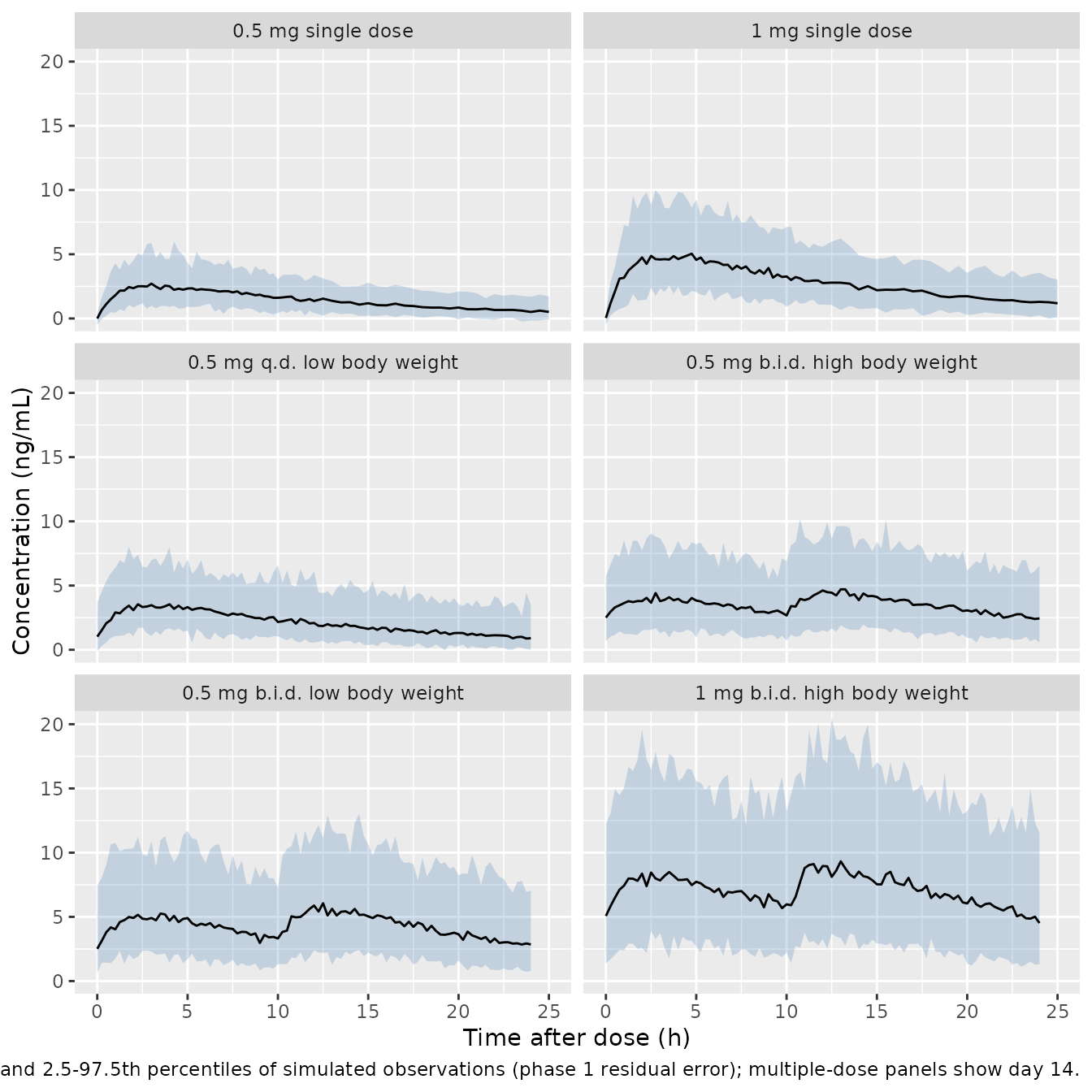

PKNCA: single-dose profiles

The paper reports no NCA table. The PKNCA run below summarises the single-dose arms and gates the typical-value solve against the model’s own closed-form identity AUC(0-inf) = 1000 x Dose / (CL/F), which a dose, unit or volume transcription error would break.

sd_ev <- events |> dplyr::filter(grepl("single", arm))
nca_input <- function(sim) {
  sim |>
    dplyr::filter(!is.na(Cc)) |>
    dplyr::mutate(Cc = pmax(Cc, 0)) |>
    dplyr::select(id, time, Cc, arm)
}
sd_sim <- sim_pk |> dplyr::filter(grepl("single", arm))
conc_obj <- PKNCA::PKNCAconc(nca_input(sd_sim), Cc ~ time | arm + id)
dose_obj <- PKNCA::PKNCAdose(
  sd_ev |> dplyr::filter(evid == 1) |> dplyr::select(id, time, amt, arm),
  amt ~ time | arm + id
)
intervals <- data.frame(start = 0, end = Inf, cmax = TRUE, tmax = TRUE,
                        aucinf.obs = TRUE, half.life = TRUE)
nca_res <- PKNCA::pk.nca(PKNCA::PKNCAdata(conc_obj, dose_obj, intervals = intervals))
summary(nca_res)
#>  start end                arm   N        cmax              tmax   half.life
#>      0 Inf 0.5 mg single dose 100 2.56 [27.6] 3.00 [1.50, 5.25] 10.6 [4.54]
#>      0 Inf   1 mg single dose 100 5.02 [23.2] 3.25 [1.75, 5.50] 10.8 [4.14]
#>   aucinf.obs
#>  46.0 [36.9]
#>  93.0 [35.7]
#> 
#> Caption: cmax, aucinf.obs: geometric mean and geometric coefficient of variation; tmax: median and range; half.life: arithmetic mean and standard deviation; N: number of subjects

# Typical 70 kg White male, 0.5 and 1 mg single dose, fine grid, tight solver
typ_ev <- data.frame(id = 1:2, WT = 70, SEXF = 0, RACE_BLACK = 0, RACE_OTHER = 0,
                     STUDY_PHASE4 = 0, arm = c("0.5 mg", "1 mg"), dose = c(0.5, 1)) |>
  merge(data.frame(time = c(0, seq(0.05, 2, by = 0.05), seq(2.25, 24, by = 0.25),
                            seq(25, 240, by = 1)))) |>
  dplyr::mutate(evid = 0L, amt = 0, cmt = "central")
typ_ev <- dplyr::bind_rows(
  typ_ev |> dplyr::distinct(id, .keep_all = TRUE) |>
    dplyr::mutate(time = 0, evid = 1L, amt = dose, cmt = "depot"),
  typ_ev
) |> dplyr::arrange(id, time, dplyr::desc(evid))
typ_sim <- rxode2::rxSolve(rxode2::zeroRe(mod_pk), typ_ev, keep = c("arm", "dose"),
                           rtol = 1e-10, atol = 1e-12, returnType = "data.frame")
#> ℹ parameter labels from comments will be replaced by 'label()'
#> Warning: No sigma parameters in the model
#> ℹ omega/sigma items treated as zero: 'etalcl', 'etalvc', 'etalka'
#> Warning: multi-subject simulation without without 'omega'
typ_nca <- PKNCA::pk.nca(PKNCA::PKNCAdata(
  PKNCA::PKNCAconc(nca_input(typ_sim), Cc ~ time | arm + id),
  PKNCA::PKNCAdose(typ_ev |> dplyr::filter(evid == 1) |> dplyr::select(id, time, amt, arm),
                   amt ~ time | arm + id),
  intervals = data.frame(start = 0, end = Inf, aucinf.obs = TRUE, cmax = TRUE, tmax = TRUE)
))
typ_tab <- as.data.frame(typ_nca$result) |>
  dplyr::filter(PPTESTCD %in% c("aucinf.obs", "cmax", "tmax")) |>
  dplyr::select(arm, PPTESTCD, PPORRES) |>
  tidyr::pivot_wider(names_from = PPTESTCD, values_from = PPORRES) |>
  dplyr::mutate(closed_form_auc = 1000 * c(0.5, 1) / 12.5)
# 240 h is ~19 half-lives, so extrapolation is negligible; the residual is
# trapezoidal error around tmax (~0.1% on this grid).
stopifnot(nrow(typ_tab) == 2,
          all(abs(typ_tab$aucinf.obs / typ_tab$closed_form_auc - 1) < 0.01))
typ_tab |>
  dplyr::rename("Dose" = arm, "Cmax (ng/mL)" = cmax, "Tmax (h)" = tmax,
                "AUC0-inf PKNCA (ng*h/mL)" = aucinf.obs,
                "1000 x Dose / CL (ng*h/mL)" = closed_form_auc) |>
  knitr::kable(digits = 2, caption = "Typical 70 kg White male, single dose.")

Typical 70 kg White male, single dose.

Dose	Cmax (ng/mL)	Tmax (h)	AUC0-inf PKNCA (ng*h/mL)	1000 x Dose / CL (ng*h/mL)
0.5 mg	1.80	3.5	40	40
1 mg	3.59	3.5	80	80

Phase 4 exposure by dose group (Figure 3, lower panels)

The box plots under Figure 3 show the empirical-Bayes AUC24 of the phase 4 varenicline subjects per dose and weight group. The medians were digitized by the maintainers from the vector graphic. The model’s individual AUC24 (daily dose / individual CL/F) in 200 simulated subjects per group with the phase 4 demographics (32.4% female; 7.9% Black; 18.7% Asian/other) is compared below.

fig3_box <- tibble::tribble(
  ~group,                           ~daily_dose, ~lo, ~hi,  ~digitized_median,
  "0.5 mg q.d. low body weight",    0.5,         35,  55,   50.2,
  "0.5 mg b.i.d. low body weight",  1.0,         35,  55,   84.1,
  "0.5 mg b.i.d. high body weight", 1.0,         55,  121,  79.5,
  "1 mg b.i.d. high body weight",   2.0,         55,  121,  152.8
)
n_grp <- 200L
auc_ev <- dplyr::bind_rows(lapply(seq_len(nrow(fig3_box)), function(k) {
  g <- fig3_box[k, ]
  d <- data.frame(id = (k - 1L) * n_grp + seq_len(n_grp), time = 0, evid = 0L,
                  amt = 0, cmt = "central", group = g$group,
                  daily_dose = g$daily_dose, WT = draw_wt(n_grp, g$lo, g$hi),
                  SEXF = stats::rbinom(n_grp, 1, 0.324), STUDY_PHASE4 = 1L)
  dplyr::bind_cols(d, draw_race(n_grp, 0.079, 0.187))
}))
auc_sim <- rxode2::rxSolve(mod_pk, auc_ev, keep = c("group", "daily_dose"),
                           returnType = "data.frame") |>
  dplyr::mutate(AUC24 = 1000 * daily_dose / cl)
auc_cmp <- auc_sim |>
  dplyr::group_by(group) |>
  dplyr::summarise(model_median = median(AUC24), .groups = "drop") |>
  dplyr::inner_join(fig3_box, by = "group") |>
  dplyr::mutate(pct_diff = 100 * (model_median / digitized_median - 1))
stopifnot(
  nrow(auc_cmp) == 4,
  # Structural gate only. The comparison is simulated individual AUC24 against
  # the medians of shrunken empirical-Bayes AUC24 in groups of unknown size and
  # weight mix, so the model sits systematically above the figure (realized
  # +2% to +20%, centre about +13%, on the development machine; see
  # Assumptions). A mis-transcribed CL/F or a unit error moves every group by
  # far more than these bounds (a 1000-fold unit slip, or CL/F off by 2x).
  abs(median(auc_cmp$pct_diff)) < 25,
  all(abs(auc_cmp$pct_diff) < 40)
)
auc_cmp |>
  dplyr::select(group, digitized_median, model_median, pct_diff) |>
  dplyr::rename("Dose group" = group, "Figure 3 median (digitized)" = digitized_median,
                "Model median" = model_median, "Difference (%)" = pct_diff) |>
  knitr::kable(digits = 1, caption = "Median AUC24 (ng*h/mL) by phase 4 dose group.")

Median AUC24 (ng*h/mL) by phase 4 dose group.

Dose group	Figure 3 median (digitized)	Model median	Difference (%)
0.5 mg b.i.d. high body weight	79.5	81.3	2.2
0.5 mg b.i.d. low body weight	84.1	101.0	20.1
0.5 mg q.d. low body weight	50.2	55.1	9.7
1 mg b.i.d. high body weight	152.8	177.7	16.3

Nausea or vomiting exposure-response

AUC_VAREN is the individual AUC24 in ng*h/mL (0 for placebo). The helper below solves the model for a data frame of covariate rows.

p_nv <- function(cov) {
  ev <- dplyr::bind_cols(data.frame(id = seq_len(nrow(cov)), time = 0, evid = 0L, amt = 0), cov)
  rxode2::rxSolve(mod_nv, ev, returnType = "data.frame")$prob_nausea_vomiting
}

Figure 4: covariate effects

Figure 4 plots the probability ratio against a representative subject (16-year-old White male, first cigarette 31-60 min after waking, AUC24 = 153 ng*h/mL). The point estimates were digitized by the maintainers from the vector graphic.

rep_subj <- data.frame(AGE = 16, SEXF = 0, RACE_BLACK = 0, RACE_OTHER = 0,
                       SMOKE_TTFC_SCORE = 1, AUC_VAREN = 153)
fig4 <- tibble::tribble(
  ~label,                        ~AGE, ~SEXF, ~RACE_BLACK, ~RACE_OTHER, ~SMOKE_TTFC_SCORE, ~digitized,
  "Age = 12 y",                    12,     0,           0,           0,                 1,     0.863,
  "Age = 17 y",                    17,     0,           0,           0,                 1,     1.035,
  "Age = 19 y",                    19,     0,           0,           0,                 1,     1.087,
  "Female",                        16,     1,           0,           0,                 1,     1.864,
  "First cig. > 60 min",           16,     0,           0,           0,                 0,     0.000,
  "First cig. within 6-30 min",    16,     0,           0,           0,                 2,     0.955,
  "First cig. < 5 min",            16,     0,           0,           0,                 3,     0.941,
  "Race (black)",                  16,     0,           1,           0,                 1,     1.234,
  "Race (other)",                  16,     0,           0,           1,                 1,     1.063
)
p_ref <- p_nv(rep_subj)
#> ℹ parameter labels from comments will be replaced by 'label()'
#> ℹ omega/sigma items treated as zero: 'etabase_logit'
fig4$model <- p_nv(dplyr::mutate(fig4[, c("AGE", "SEXF", "RACE_BLACK", "RACE_OTHER",
                                           "SMOKE_TTFC_SCORE")], AUC_VAREN = 153)) / p_ref
#> ℹ omega/sigma items treated as zero: 'etabase_logit'
#> Warning: multi-subject simulation without without 'omega'
# Deterministic; the digitized points sit 0.003-0.008 above the model on every
# row (a constant plotting offset), so 0.015 leaves headroom and still catches
# any mis-transcribed factor.
stopifnot(nrow(fig4) == 9, all(abs(fig4$model - fig4$digitized) < 0.015),
          abs(fig4$model[fig4$label == "Female"] - 1.86) < 0.01)
fig4 |>
  dplyr::select(label, digitized, model) |>
  dplyr::rename("Covariate" = label, "Figure 4 (digitized)" = digitized,
                "Model" = model) |>
  knitr::kable(digits = 3, caption = paste0(
    "Probability ratio vs the representative subject (model p = ",
    signif(p_ref, 3), ")."))

Probability ratio vs the representative subject (model p = 0.284).

Covariate	Figure 4 (digitized)	Model
Age = 12 y	0.863	0.859
Age = 17 y	1.035	1.030
Age = 19 y	1.087	1.084
Female	1.864	1.856
First cig. > 60 min	0.000	0.000
First cig. within 6-30 min	0.955	0.950
First cig. < 5 min	0.941	0.937
Race (black)	1.234	1.229
Race (other)	1.063	1.057

The Results statement of an “~86%” increase for female smokers is reproduced (ratio 1.856). The very small probability at “first cigarette > 60 min” is the model reference level: its intercept of -30.9 is scaled by about 0.075-0.078 for every other level, and only 5 of the 238 subjects were in it.

Figure 3b: probability versus exposure

The Figure 3b ‘Model predicted’ line is not a single logistic curve; it closely matches the model’s predicted probability averaged over the covariate mix of the phase 4 ER cohort (Table 2), which is what is computed below on a deterministic grid of covariate combinations (age from a normal distribution with the Table 2 mean 15.8 and SD 1.81 years, discretised on 12-20 years).

fig3b <- data.frame(
  AUC = c(5, 25, 50, 75, 100, 125, 150, 175, 200, 225, 250, 275, 300),
  digitized = c(0.127, 0.153, 0.181, 0.220, 0.264, 0.309, 0.354, 0.399, 0.444,
                0.490, 0.536, 0.582, 0.629)
)
age_grid <- data.frame(AGE = seq(12, 20, by = 0.25))
age_grid$w_age <- stats::dnorm(age_grid$AGE, 15.8, 1.81)
age_grid$w_age <- age_grid$w_age / sum(age_grid$w_age)
cov_grid <- tidyr::crossing(
  data.frame(SMOKE_TTFC_SCORE = 0:3, w_ttfc = c(5, 39, 96, 98) / 238),
  data.frame(SEXF = 0:1, w_sex = c(157, 81) / 238),
  data.frame(RACE_BLACK = c(0, 1, 0), RACE_OTHER = c(0, 0, 1),
             w_race = c(176, 16, 46) / 238),
  age_grid,
  data.frame(AUC_VAREN = fig3b$AUC)
) |>
  dplyr::mutate(w = w_ttfc * w_sex * w_race * w_age)
cov_grid$p <- p_nv(cov_grid[, c("AGE", "SEXF", "RACE_BLACK", "RACE_OTHER",
                                "SMOKE_TTFC_SCORE", "AUC_VAREN")])
#> ℹ omega/sigma items treated as zero: 'etabase_logit'
#> Warning: multi-subject simulation without without 'omega'
avg <- cov_grid |>
  dplyr::group_by(AUC = AUC_VAREN) |>
  dplyr::summarise(model = sum(w * p) / sum(w), .groups = "drop") |>
  dplyr::inner_join(fig3b, by = "AUC")
# Deterministic. Realized maximum 0.022 (at AUC 300, beyond most of the data);
# 0.035 still catches a slope or intercept error, which moves the curve by
# more than 0.1.
stopifnot(nrow(avg) == nrow(fig3b), max(abs(avg$model - avg$digitized)) < 0.035)
ggplot(avg, aes(AUC)) +
  geom_line(aes(y = model, linetype = "Model (cohort-averaged)")) +
  geom_point(aes(y = digitized, shape = "Figure 3b line (digitized)")) +
  coord_cartesian(ylim = c(0, 1)) +
  labs(x = "AUCss(0-24) (ng*h/mL)", y = "Probability of nausea/vomiting",
       linetype = NULL, shape = NULL,
       caption = "Replicates the model line of Figure 3b of Fediuk 2021.")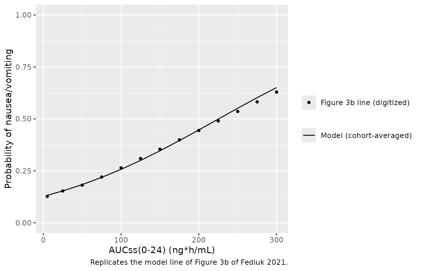

Continuous abstinence, weeks 9-12

The paper reports this model only through Figure 3a and its slope p-value (0.303). The dotted ‘Model predicted’ line is a straight line in probability, from 0.192 at AUC24 = 0 to 0.320 at the largest observed AUC24 (about 314 ng*h/mL). The packaged logistic was fitted by the maintainers to that line (see Assumptions); the check below confirms it stays on the drawn line.

fig3a <- data.frame(
  AUC = c(5, 25, 50, 75, 100, 125, 150, 175, 200, 225, 250, 275, 300),
  digitized = c(0.194, 0.202, 0.212, 0.221, 0.231, 0.241, 0.251, 0.261, 0.271,
                0.281, 0.291, 0.301, 0.311)
)
fig3a$model <- rxode2::rxSolve(
  mod_car,
  data.frame(id = seq_len(nrow(fig3a)), time = 0, evid = 0L, amt = 0,
             AUC_VAREN = fig3a$AUC),
  returnType = "data.frame"
)$p_car
#> Warning: multi-subject simulation without without 'omega'
# Deterministic; realized maximum 0.0023.
stopifnot(max(abs(fig3a$model - fig3a$digitized)) < 0.01)
# Observed binned proportions from Figure 3a (digitized), for context only.
obs3a <- data.frame(AUC = c(0, 54.9, 73.1, 89.5, 136.5, 174.6, 227.1),
                    p = c(0.181, 0.199, 0.249, 0.199, 0.278, 0.333, 0.248))
ggplot(fig3a, aes(AUC)) +
  geom_line(aes(y = model, linetype = "Packaged model")) +
  geom_point(aes(y = digitized, shape = "Figure 3a line (digitized)")) +
  geom_point(data = obs3a, aes(y = p, shape = "Observed bins (digitized)")) +
  scale_shape_manual(values = c(16, 1)) +
  coord_cartesian(ylim = c(0, 1)) +
  labs(x = "AUCss(0-24) (ng*h/mL)", y = "Probability of CAR9-12",
       linetype = NULL, shape = NULL,
       caption = "Replicates Figure 3a of Fediuk 2021.")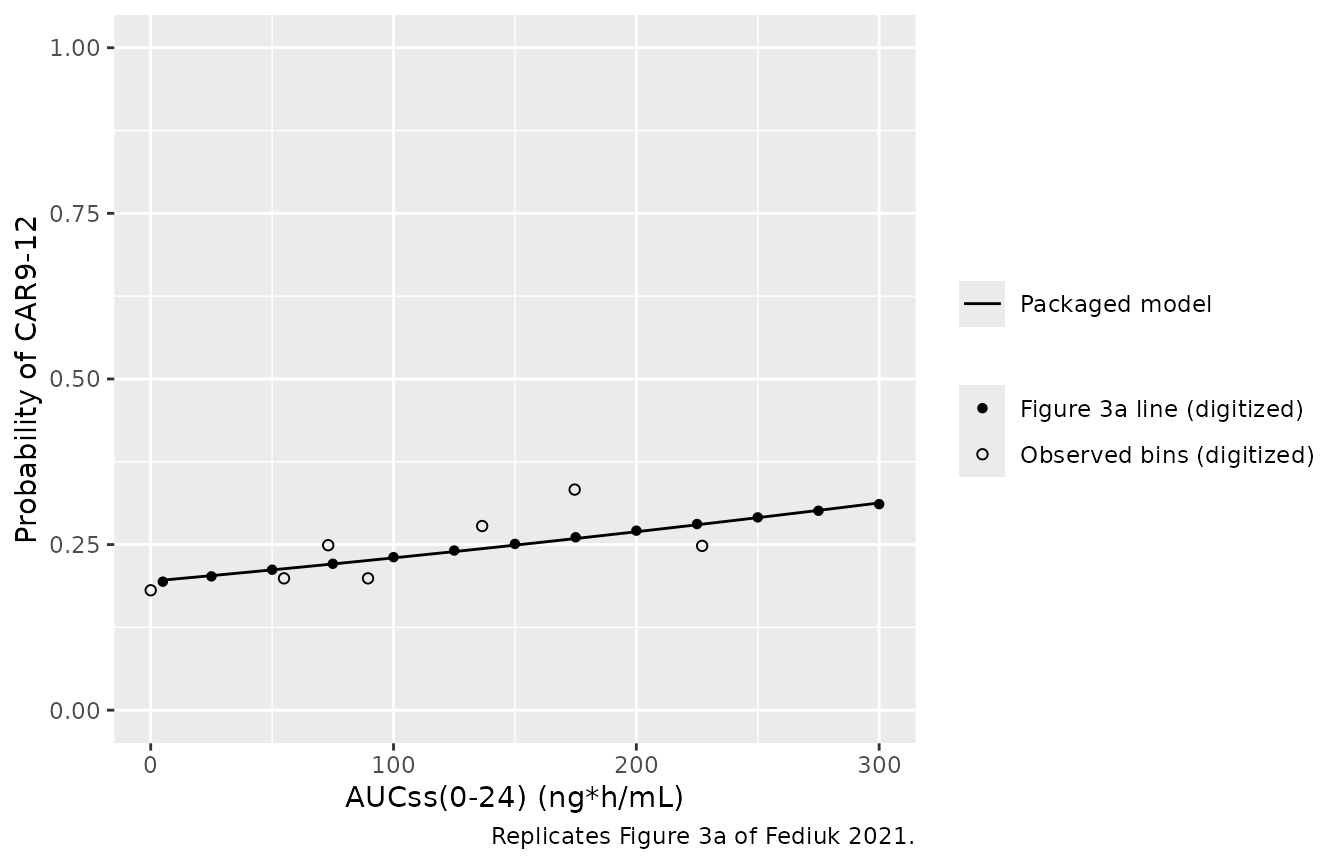

Assumptions and deviations

• CAR9-12 parameters are digitized, not published. Fediuk 2021 gives no estimates for the CAR9-12 model (Table S2 and Text S2 cover the nausea/vomiting model only) and states only that the AUC24 slope was not significant (p = 0.303) so no covariates were added. The maintainers extracted the dotted ‘Model predicted’ line of Figure 3a from the article’s vector graphics (99 dash segments, axes mapped on the printed ticks) and fitted logit(p) = base_logit + slope x AUC24 to it on the logit scale, giving -1.42 and 0.00211 per ngh/mL. The drawn line is exactly straight in probability, which a logistic curve cannot be, so the plot was probably drawn through two predicted points; the fitted logistic stays within 0.003 of it over the observed exposure range (0-314 ngh/mL). Treat the slope as a figure approximation with no uncertainty estimate, and do not extrapolate beyond that range.
• Figure 2 and Figure 4 values. Figure 2 ratios are printed in the figure and were read from the PDF text. Figure 4 prints no numbers; its point estimates, the Figure 3 exposure-box medians and the Figure 3a/3b lines were digitized by the maintainers from the vector graphics (reading precision about 0.005 on the ratio axis).
• Placeholder residual on the ER models. The ER models were fitted with a Bernoulli likelihood (Text S2 Y = P**DV*(1-P)**(1-DV)), which has no residual-error parameter. Both ER files expose the deterministic probability with a fixed additive SD of 0.001 so the model can be declared; draw binary outcomes externally with rbinom(n, 1, p).
• Between-subject variance of the nausea/vomiting logit is fixed(0), as in Text S2 ($OMEGA 0 FIX, naive-pooled analysis).
• Residual error stratum. The phase 1 and phase 4 studies have separate residual errors, selected by the new STUDY_PHASE4 column (0 = phase 1, 1 = phase 4). It does not change typical-value predictions. The Figure 1 replicate uses the phase 1 values.
• Omega covariances. Table 3 prints the CL/F-V/F and CL/F-ka covariances as -0.00162 and -0.0582, while the Text S1 $OMEGA block (the initial values of the final run) prints -0.00161 and -0.0581; the Table 3 final estimates are used.
• Reported %CV of the IIV. Results quotes 32%, 13% and 44% for CL/F, V/F and ka. These mix conventions: 32% and 13% match sqrt(omega^2) (31.9%, 13.5%) while 44% matches sqrt(exp(omega^2) - 1) (43.6%). The packaged variances are the Table 3 omega^2 values, which are unambiguous.
• Bid dosing interval. The evening dose is given 10 h after the morning dose in the Figure 1 replicate (Table 1 note c for the multiple-dose phase 1 study); titration is not simulated, and the plotted day-14 profile is at steady state.
• Virtual cohorts. Body weight is drawn from a normal distribution with the pooled Table 2 mean and SD and redrawn into each weight band; race and sex follow the Table 2 proportions.
• Phase 4 exposure by dose group is not closely reproduced. The simulated median AUC24 is above the digitized Figure 3 box-plot median in all four groups (about +2% for 0.5 mg b.i.d. high body weight up to about +20% for 0.5 mg b.i.d. low body weight). Figure 3 plots empirical-Bayes estimates for the phase 4 subjects, whose per-group size, weight and race mix are not reported, and those estimates are shrunk toward the population (CL/F shrinkage 30.6%); the virtual cohort can only approximate that mix. The typical-value checks against Figure 2 and the Discussion, which do not depend on a cohort, are reproduced exactly. The gate in that section is therefore structural only (it catches a unit or clearance transcription error).
• Covariates not in the final PK model. Age and creatinine clearance were deliberately not tested because both correlate with body weight (Methods); they are documented in covariatesDataExcluded.
• No correction notice was found for this article (EuropePMC and the publisher page, checked 2026-09-28).