Alectinib (van der Heijden 2023)
Source:vignettes/articles/vanderHeijden_2023_alectinib.Rmd
vanderHeijden_2023_alectinib.RmdModel and source
- Citation: van der Heijden LT, Steeghs N, Beijnen JH, Huitema ADR, Dorlo TPC. The use of microtracers in food-effect trials: An alternative study design for toxic drugs with long half-lives exemplified by the case for alectinib. Clin Transl Sci. 2023;16:2557-2564. doi:10.1111/cts.13647. Structural model and estimates from the European Medicines Agency (EMA) Alecensa Assessment Report (2016), as reproduced in the paper’s Data S1 (Table S2 and NONMEM code).
- Description: One-compartment population PK model for oral alectinib (an ALK inhibitor) in adults with ALK-positive non-small cell lung cancer, used by van der Heijden 2023 to simulate a stable-isotope-labelled microtracer (alectinib-d6) food-effect study during steady-state alectinib treatment. The structural model and its estimates are the European Medicines Agency Alecensa assessment-report model (138 patients, 600 mg twice daily with a meal): sequential zero-order input into the depot over D1 = 3.44 h followed by first-order absorption at ka = 1.30 1/h, CL/F = 81.9 L/h and V/F = 4016 L, each allometrically scaled by body weight (exponents 0.75 and 1, reference 70 kg). Relative bioavailability is 1 for a dose taken with food and 0.714 fasted (the assumed 40% food effect), with an assumed 8% (CV) between-occasion variability on bioavailability. Correlated between-subject variability on CL/F and V/F, independent variability on ka and D1, and a proportional residual error of 19%; the assessment-report model’s additive error is dropped for the microtracer concentration range.
- Article: https://doi.org/10.1111/cts.13647 (open access; the parameter table and NONMEM code are in the article’s Data S1)
van der Heijden 2023 did not fit a model to data. It asked whether a stable-isotope-labelled microtracer (100 ug alectinib-d6), given once with a standardized meal and once fasted to patients already at steady state on alectinib, could detect a 40% food effect on bioavailability. To answer it the authors simulated microtracer concentrations with the population PK model of the European Medicines Agency (EMA) Alecensa assessment report, to which they added a fixed food effect on bioavailability and between-occasion variability (IOV) on bioavailability, and then ran stochastic simulation and estimation (1000 trials per design) in NONMEM. This package ships that simulation model.
Population
The structural model and its estimates come from 138 patients with locally advanced or metastatic ALK-positive non-small cell lung cancer in the pooled pivotal phase II studies NP28673 and NP28761, all of whom received alectinib 600 mg twice daily with a meal (Data S1 Table S1). Median age was 52 years (range 22-79); 56% were female; 67% White, 26% Asian, 0.7% Black or African American, 0.7% American Indian or Alaska Native, 3% other and 2% unknown. 61% had CNS metastases, 95% had adenocarcinoma and 80% had received prior chemotherapy. Body weight was not tabulated for this cohort; the trial simulations resampled weight from a previous alectinib NSCLC cohort (median 77.5 kg, range 49-123 kg).
The same information is available programmatically via
readModelDb("vanderHeijden_2023_alectinib")()$population.
Source trace
Every ini() value carries an in-file comment in
inst/modeldb/specificDrugs/vanderHeijden_2023_alectinib.R.
All values are in Data S1 Table S2, which the article reproduces from
the EMA assessment report (structural and IIV estimates) plus the two
simulation assumptions marked with an asterisk there (fasted
bioavailability and IOV).
| Equation / parameter | Value | Source location |
|---|---|---|
lcl (CL/F at 70 kg) |
log(81.9 L/h) | Table S2 ‘Cl/F’; $THETA(1) |
lvc (V/F at 70 kg) |
log(4016 L) | Table S2 ‘V/F’; $THETA(2) |
lka |
log(1.30 1/h) | Table S2 ‘Ka’; $THETA(3) |
ld1 (zero-order input duration) |
log(3.44 h) | Table S2 ‘D1’; $THETA(4) |
e_wt_cl, e_wt_vc
|
0.75, 1 (fixed) | Methods ‘Population pharmacokinetic model’; Data S1 code TVCL / TVV |
lfdepot (F with food) |
log(1) (fixed) | Table S2 ‘F (fed conditions)’; $THETA(5) 1 FIX |
lfdepot_fasted (F fasted) |
log(0.714) (fixed) | Table S2 ‘F (fasted conditions)’; Methods |
etalcl, etalvc block |
0.162, 0.07865012, 0.161 | Table S2 IIV rows and covariance; $OMEGA BLOCK(2) |
etalka, etald1
|
0.398, 0.178 | Table S2 ‘IIV Ka’, ‘IIV D1’ |
etaiov_fdepot_1, etaiov_fdepot_2
|
0.0064 each (fixed) | Table S2 ‘IOV’; $OMEGA BLOCK(1) + BLOCK(1) SAME | | `propSd` | 0.19 | Table S2 'Proportional error' = 0.0361 (variance) | | CL, V allometry `(WT/70)^e` | n/a | Data S1 code `TVCL = THETA(1)*(WT/70)**0.75`, `TVV = THETA(2)*(WT/70)**1` | | F by prandial state and occasion | n/a | Data S1 code `F1=THETA(5)*EXP(ETA(OCC_F1))`; `IF(FLAG.EQ.1) F1=THETA(6)*EXP(ETA(OCC_F1))` | | Sequential zero-order then first-order absorption | n/a | Methods; Data S1 `ADVAN2 TRANS2` with `D1` | | `Cc ~ prop(propSd)` | n/a | Data S1 `$ERROR Y = F*(1+EPS(1))+EPS(2)` with EPS(2) 0 FIX |
Typical-value checks
Doses go into depot with rate = -2, so the
dose enters the depot at a constant rate over the modelled duration
D1 before first-order absorption.
mod <- readModelDb("vanderHeijden_2023_alectinib")
mod_typ <- rxode2::zeroRe(mod)
#> ℹ parameter labels from comments will be replaced by 'label()'
#> Warning: some etas defaulted to non-mu referenced, possible parsing error: etaiov_fdepot_1, etaiov_fdepot_2
#> as a work-around try putting the mu-referenced expression on a simple line
#> Warning: some etas defaulted to non-mu referenced, possible parsing error: etaiov_fdepot_1, etaiov_fdepot_2
#> as a work-around try putting the mu-referenced expression on a simple line

typ_events <- function(amt, fed, occ, id) {
  tibble(
    id = id,
    time = c(0, seq(0, 480, by = 0.25)),
    evid = c(1L, rep(0L, length(seq(0, 480, by = 0.25)))),
    amt = c(amt, rep(0, length(seq(0, 480, by = 0.25)))),
    rate = c(-2, rep(0, length(seq(0, 480, by = 0.25)))),
    cmt = "depot",
    WT = 70,
    FED = fed,
    OCC = occ
  )
}

ev_typ <- bind_rows(
  typ_events(0.1, fed = 1, occ = 1, id = 1L) |> mutate(prandial = "Fed"),
  typ_events(0.1, fed = 0, occ = 2, id = 2L) |> mutate(prandial = "Fasted")
)
sim_typ <- rxode2::rxSolve(
  mod_typ, events = ev_typ, keep = "prandial", rtol = 1e-10, atol = 1e-12
) |>
  as.data.frame()
#> ℹ omega/sigma items treated as zero: 'etalcl', 'etalvc', 'etalka', 'etald1', 'etaiov_fdepot_1', 'etaiov_fdepot_2'
#> Warning: multi-subject simulation without without 'omega'

auc_trap <- function(t, y) sum(diff(t) * (head(y, -1) + tail(y, -1)) / 2)
typ_summary <- sim_typ |>
  group_by(prandial) |>
  summarise(
    cmax_pg = 1000 * max(Cc),
    tmax = time[which.max(Cc)],
    auc = auc_trap(time, Cc),
    .groups = "drop"
  )
auc_fed <- typ_summary$auc[typ_summary$prandial == "Fed"]
auc_fasted <- typ_summary$auc[typ_summary$prandial == "Fasted"]
fe_typ <- 100 * (auc_fed - auc_fasted) / auc_fasted
t_half <- log(2) * 4016 / 81.9

typ_summary |>
  dplyr::rename(
    "Prandial state" = prandial,
    "Cmax (pg/mL)" = cmax_pg,
    "Tmax (h)" = tmax,
    "AUC0-480 (ng*h/mL)" = auc
  ) |>
  knitr::kable(
    digits = 3,
    caption = "Typical 70-kg patient, single 100 ug microtracer dose."
)| Prandial state | Cmax (pg/mL) | Tmax (h) | AUC0-480 (ng*h/mL) |
|---|---|---|---|
| Fasted | 16.451 | 5.5 | 0.872 |
| Fed | 23.041 | 5.5 | 1.221 |
For a typical 70-kg patient the model gives:
- a food effect of 40.06% on AUC, the 40% the authors defined as minimally clinically relevant (Equation 1, FE = (1 - 0.714)/0.714 = 40%);
- a terminal half-life of log(2) x V/CL = 34 h, close to the 32 h the article cites for alectinib;
- Tmax of 5.5 h, inside the 4-6 h window the article uses to place its absorption-phase samples;
- a fed microtracer Cmax of about 23 pg/mL, the ‘pg/mL’ range the Methods give as the reason the additive error was dropped.
stopifnot(
  # Food effect is fixed by construction; the solve reproduces the 40%
  # through F1 = 1 fed vs 0.714 fasted (tolerance covers the 480 h window).
  abs(fe_typ - 40.06) < 0.1,
  # AUC equals F * Dose / CL (dose in mg -> ng/mL via the x1000).
  abs(auc_fed / (0.1 * 1000 / 81.9) - 1) < 0.01,
  all(typ_summary$tmax >= 4 & typ_summary$tmax <= 6),
  abs(t_half - 32) / 32 < 0.1
)
Therapeutic steady state
The microtracer is given on top of the patients’ 600 mg twice-daily alectinib taken with food. The proposed design requires at least 7 days of treatment before the first microtracer dose, which is about five half-lives.
ev_ss <- rxode2::et(amt = 600, ii = 12, addl = 27, cmt = "depot", rate = -2) |>
  rxode2::et(seq(0, 336, by = 0.5)) |>
  as.data.frame() |>
  mutate(WT = 70, FED = 1, OCC = 0)

sim_ss <- rxode2::rxSolve(mod_typ, events = ev_ss) |> as.data.frame()
#> ℹ omega/sigma items treated as zero: 'etalcl', 'etalvc', 'etalka', 'etald1', 'etaiov_fdepot_1', 'etaiov_fdepot_2'

troughs <- sim_ss |> filter(time %in% seq(12, 336, by = 12))
frac_ss_day7 <- troughs$Cc[troughs$time == 168] / troughs$Cc[troughs$time == 336]
stopifnot(frac_ss_day7 > 0.9, frac_ss_day7 < 1)

ggplot(sim_ss, aes(time / 24, Cc)) +
  geom_line() +
  geom_vline(xintercept = 7, linetype = "dashed") +
  labs(
    x = "Time (days)",
    y = "Alectinib Cc (ng/mL)",
    title = "Typical 70-kg patient, alectinib 600 mg twice daily with food",
    caption = "Dashed line: day 7, the minimum treatment duration before the microtracer study."
  )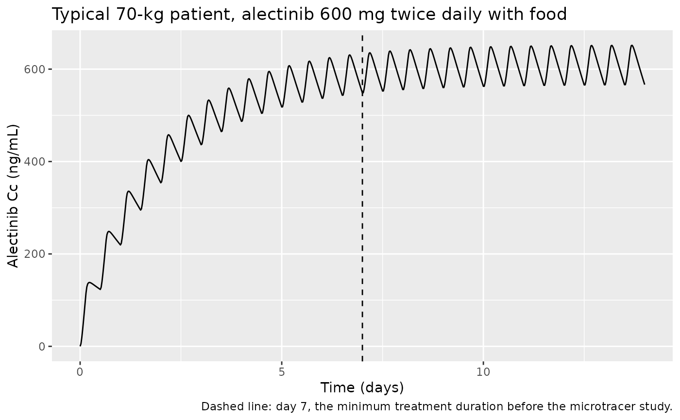
The day-7 trough is 96.9% of the day-14 trough.
Virtual cohort and proposed study design
The proposed design (Figure 1c) gives the microtracer with food on
study day 1 (OCC = 1, FED = 1) and fasted on
study day 9 (OCC = 2, FED = 0), with samples
at predose and 0.5, 1, 1.5, 2, 4, 6, 8, 10, 12 and 24 h after each
microtracer dose. One trial has 10 patients; 20 trials (200 patients)
are simulated here. Body weight is drawn from a log-normal centred on
the article’s resampling cohort median (77.5 kg) and truncated to its
49-123 kg range.
The random effects are drawn in base R and passed to the
typical-value model through params, so the cohort is
identical on every machine and the same patient carries the same
between-subject random effects on both occasions.
set.seed(20231012)
n_trials <- 20L
n_per_trial <- 10L
n_sub <- n_trials * n_per_trial

omega <- rxode2::rxode2(mod)$omega
#> ℹ parameter labels from comments will be replaced by 'label()'
#> Warning: some etas defaulted to non-mu referenced, possible parsing error: etaiov_fdepot_1, etaiov_fdepot_2
#> as a work-around try putting the mu-referenced expression on a simple line
eta <- matrix(rnorm(n_sub * nrow(omega)), n_sub) %*% chol(omega)
colnames(eta) <- rownames(omega)

wt <- exp(rnorm(n_sub * 3, log(77.5), 0.2))
wt <- head(wt[wt >= 49 & wt <= 123], n_sub)
stopifnot(length(wt) == n_sub)

subjects <- tibble(
  id = seq_len(n_sub),
  trial = rep(seq_len(n_trials), each = n_per_trial),
  WT = wt
)
params <- data.frame(id = subjects$id, eta)

sample_times <- c(0, 0.5, 1, 1.5, 2, 4, 6, 8, 10, 12, 24)
design_events <- bind_rows(
  # Day 1: microtracer with food
  subjects |> mutate(time = 0, evid = 1L, amt = 0.1, rate = -2, FED = 1, OCC = 1),
  subjects |> tidyr::expand_grid(time = sample_times) |>
    mutate(evid = 0L, amt = 0, rate = 0, FED = 1, OCC = 1),
  # Day 9: microtracer fasted
  subjects |> mutate(time = 192, evid = 1L, amt = 0.1, rate = -2, FED = 0, OCC = 2),
  subjects |> tidyr::expand_grid(time = 192 + sample_times[-1]) |>
    mutate(evid = 0L, amt = 0, rate = 0, FED = 0, OCC = 2)
) |>
  mutate(cmt = "depot") |>
  arrange(id, time, desc(evid))

sim_design <- rxode2::rxSolve(
  mod_typ, events = design_events, params = params, keep = "trial"
) |>
  as.data.frame() |>
  mutate(
    occasion = ifelse(OCC == 1, "Day 1, fed", "Day 9, fasted"),
    tad = ifelse(OCC == 1, time, time - 192)
  )
#> Warning: multi-subject simulation without without 'omega'
# Proposed design of Figure 1c: microtracer concentration-time profiles on
# the two sampling days (individual predictions, 200 patients).
sim_design |>
  group_by(occasion, tad) |>
  summarise(
    Q10 = quantile(1000 * Cc, 0.1),
    Q50 = quantile(1000 * Cc, 0.5),
    Q90 = quantile(1000 * Cc, 0.9),
    .groups = "drop"
  ) |>
  ggplot(aes(tad, Q50, colour = occasion, fill = occasion)) +
  geom_ribbon(aes(ymin = Q10, ymax = Q90), alpha = 0.2, colour = NA) +
  geom_line() +
  geom_point() +
  labs(
    x = "Time after microtracer dose (h)",
    y = "Alectinib-d6 Cc (pg/mL)",
    colour = NULL, fill = NULL,
    title = "Microtracer profiles under the proposed study design",
    caption = "Median and 10th-90th percentiles; sampling times of Figure 1c."
  )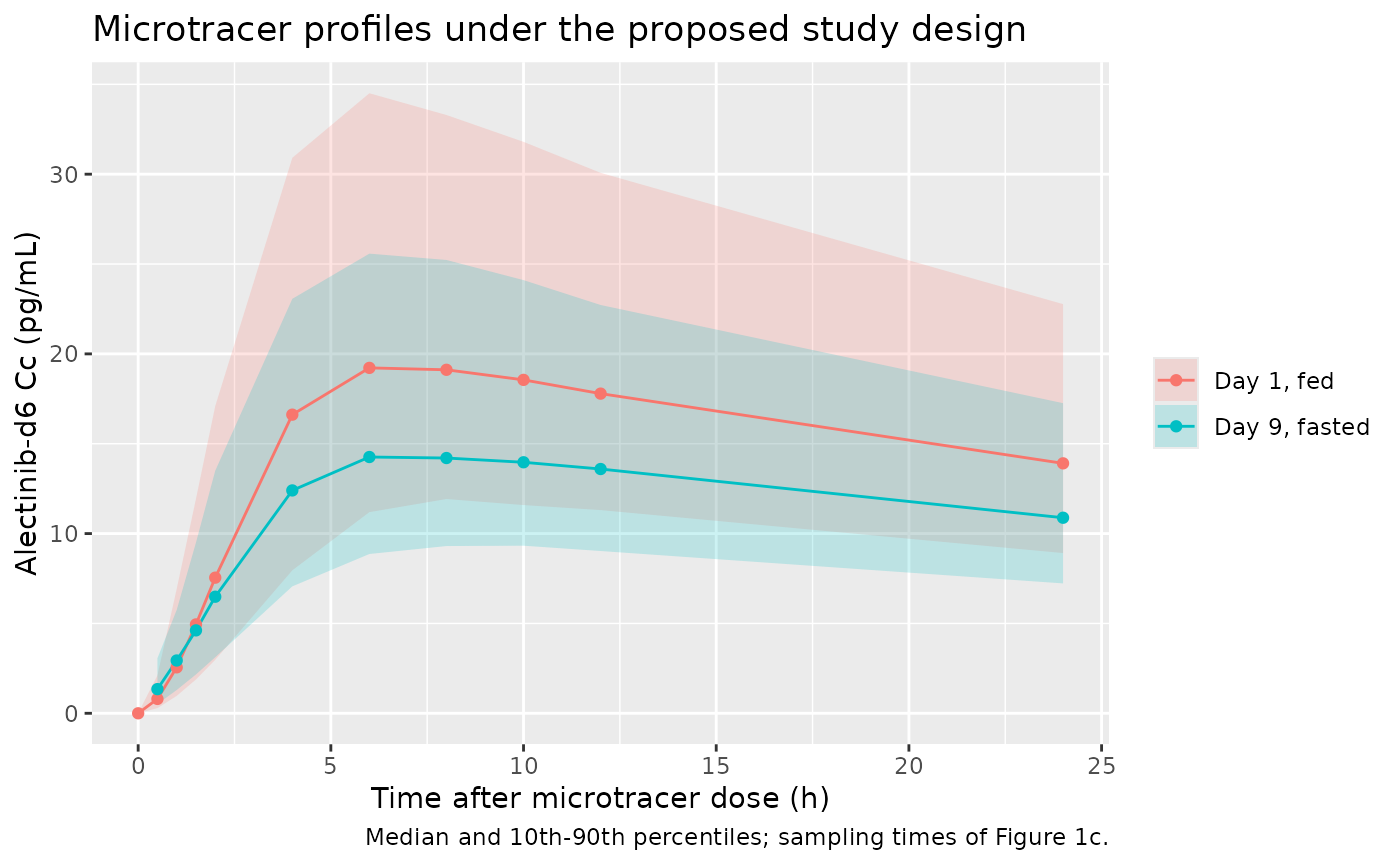
The day-9 predose sample is not zero: about 2% of the day-1 microtracer remains after the 8-day washout (5.6 half-lives). The article’s popPK analysis models both doses together, so the carry-over is accounted for; the NCA below avoids it by solving each occasion as a separate single dose.
PKNCA validation
The article reports no NCA. Its central quantity is the food effect, which under linear PK equals the ratio of dose-normalised AUCs in the same patient. Each patient is therefore solved twice as a single microtracer dose, once fed on occasion 1 and once fasted on occasion 2, with the same between-subject random effects and that occasion’s IOV random effect. AUC0-inf is computed by PKNCA per patient and occasion, and the food effect per patient is FE = AUC(fed) / AUC(fasted) - 1.
nca_times <- c(0, 0.5, 1, 1.5, 2, 3, 4, 5, 6, 8, 10, 12, 16, 24, 36, 48, 72, 96, 120, 168, 240)
single_dose <- function(fed, occ, offset) {
  bind_rows(
    subjects |> mutate(time = 0, evid = 1L, amt = 0.1, rate = -2),
    subjects |> tidyr::expand_grid(time = nca_times) |>
      mutate(evid = 0L, amt = 0, rate = 0)
  ) |>
    mutate(
      subject = id, id = id + offset, cmt = "depot", FED = fed, OCC = occ,
      treatment = ifelse(fed == 1, "Fed", "Fasted")
    ) |>
    arrange(id, time, desc(evid))
}
nca_events <- bind_rows(
  single_dose(fed = 1, occ = 1, offset = 0L),
  single_dose(fed = 0, occ = 2, offset = n_sub)
)
stopifnot(!anyDuplicated(unique(nca_events[, c("id", "time", "evid")])))

nca_params <- bind_rows(params, params |> mutate(id = id + n_sub))
sim_nca <- rxode2::rxSolve(
  mod_typ, events = nca_events, params = nca_params,
  keep = c("subject", "trial", "treatment")
) |>
  as.data.frame()
#> Warning: multi-subject simulation without without 'omega'

conc_df <- sim_nca |>
  dplyr::filter(!is.na(Cc)) |>
  dplyr::select(id, subject, trial, treatment, time, Cc)
dose_df <- nca_events |>
  dplyr::filter(evid == 1) |>
  dplyr::select(id, subject, trial, treatment, time, amt)

conc_obj <- PKNCA::PKNCAconc(conc_df, Cc ~ time | treatment + id)
dose_obj <- PKNCA::PKNCAdose(dose_df, amt ~ time | treatment + id)
intervals <- data.frame(
  start = 0, end = Inf,
  cmax = TRUE, tmax = TRUE, aucinf.obs = TRUE, half.life = TRUE
)
nca_res <- PKNCA::pk.nca(PKNCA::PKNCAdata(conc_obj, dose_obj, intervals = intervals))

nca_wide <- as.data.frame(nca_res) |>
  dplyr::filter(PPTESTCD %in% c("cmax", "tmax", "aucinf.obs", "half.life")) |>
  dplyr::select(treatment, id, PPTESTCD, PPORRES) |>
  tidyr::pivot_wider(names_from = PPTESTCD, values_from = PPORRES)

nca_wide |>
  group_by(treatment) |>
  summarise(
    cmax_pg = 1000 * median(cmax),
    tmax = median(tmax),
    aucinf = median(aucinf.obs),
    half_life = median(half.life),
    .groups = "drop"
  ) |>
  dplyr::rename(
    "Prandial state" = treatment,
    "Median Cmax (pg/mL)" = cmax_pg,
    "Median Tmax (h)" = tmax,
    "Median AUC0-inf (ng*h/mL)" = aucinf,
    "Median half-life (h)" = half_life
  ) |>
knitr::kable(digits = 3, caption = "PKNCA results, single 100 ug microtracer dose (200 patients).")| Prandial state | Median Cmax (pg/mL) | Median Tmax (h) | Median AUC0-inf (ng*h/mL) | Median half-life (h) |
|---|---|---|---|---|
| Fasted | 14.015 | 6 | 0.815 | 34.769 |
| Fed | 19.846 | 6 | 1.150 | 34.769 |
Comparison against published values
The only NCA-type value the article states for alectinib is its 32 h half-life (cited from the literature, not computed by the article).
published <- tibble::tribble(
  ~treatment, ~half.life,
  "Fed", 32,
  "Fasted", 32
)
cmp <- nlmixr2lib::ncaComparisonTable(
  simulated = nca_res,
  reference = published,
  by = "treatment",
  units = c(half.life = "h"),
  tolerance_pct = 20
)
knitr::kable(cmp, caption = "Simulated vs. published half-life. * differs from reference by >20%.")| NCA parameter | treatment | Reference | Simulated | % diff |
|---|---|---|---|---|
| t½ (h) | Fed | 32 | 34.8 | +8.7% |
| t½ (h) | Fasted | 32 | 34.8 | +8.7% |
Food effect per trial
The article’s base design (10 patients, food effect 40%, IOV 8%) estimated a mean food effect of 39.8% with an 80% interval of 31.0%-48.6% over 1000 NONMEM re-estimations (Results, ‘Feasibility study’). The NCA analogue below takes the geometric-mean AUC ratio of each simulated 10-patient trial.
fe_subject <- nca_wide |>
  dplyr::mutate(subject = ifelse(treatment == "Fed", id, id - n_sub)) |>
  dplyr::select(subject, treatment, aucinf.obs) |>
  tidyr::pivot_wider(names_from = treatment, values_from = aucinf.obs) |>
  dplyr::left_join(subjects |> dplyr::select(subject = id, trial), by = "subject") |>
  dplyr::mutate(log_ratio = log(Fed / Fasted))

fe_trial <- fe_subject |>
  group_by(trial) |>
  summarise(fe = 100 * (exp(mean(log_ratio)) - 1), .groups = "drop")

fe_table <- tibble(
  Source = c("van der Heijden 2023 (popPK SSE, 1000 trials)", "This simulation (NCA, 20 trials)"),
  `Mean FE (%)` = c(39.8, mean(fe_trial$fe)),
  `10th percentile (%)` = c(31.0, unname(quantile(fe_trial$fe, 0.1))),
  `90th percentile (%)` = c(48.6, unname(quantile(fe_trial$fe, 0.9)))
)
knitr::kable(fe_table, digits = 1, caption = "Estimated food effect per 10-patient trial.")| Source | Mean FE (%) | 10th percentile (%) | 90th percentile (%) |
|---|---|---|---|
| van der Heijden 2023 (popPK SSE, 1000 trials) | 39.8 | 31.0 | 48.6 |
| This simulation (NCA, 20 trials) | 38.8 | 33.6 | 45.9 |
stopifnot(
  nrow(fe_subject) == n_sub,
  # Centre: a reversed FED coding gives about -29%, a missing F1 effect 0%.
  abs(mean(fe_trial$fe) - 40) < 4,
  # Per-patient ratio spread comes from IOV alone: sd(log ratio) is
  # sqrt(2 * 0.0064) = 0.113; dropping or doubling the IOV moves it far
  # outside this window.
  abs(sd(fe_subject$log_ratio) - 0.113) < 0.03
)
The NCA food effect is centred on 40%, as the article’s estimate is. Its interval is narrower because the NCA uses noise-free individual predictions on a rich schedule, so the only source of spread is the 8% IOV; the article’s interval also carries the 19% proportional residual error and the uncertainty of estimating the food effect from 10 sparse profiles.
Assumptions and deviations
- The article fitted no model of its own. The structural parameters and IIV are the EMA Alecensa assessment-report estimates as reproduced in the article’s Data S1 Table S2; the EMA report itself was not consulted.
- The fasted bioavailability (0.714) and the IOV variance (0.0064, 8%
CV) are design assumptions of the simulation, not estimates, and are
fixed in the model. The article’s sensitivity analyses vary them (food
effect 20-40%, IOV 8-27%); to explore those scenarios, override
lfdepot_fastedand the twoetaiov_fdepot_*variances withini(). - The EMA model’s additive residual error was set to 0 by the authors because the microtracer concentrations (pg/mL) are far below the therapeutic range; it is omitted here and its EMA value is not reported in the article. For therapeutic alectinib concentrations the model therefore lacks the additive component of the original EMA model.
- The article assumes the microtracer (alectinib-d6) has the same PK as alectinib, so the model describes both. Its metabolite M4 is not modelled.
- The paper’s
FLAGcolumn (1 = fasted occasion) is encoded asFED = 1 - FLAG. Doses must userate = -2so the modelled durationD1is applied. - The covariance of the CL/F and V/F random effects uses the unrounded value in the Data S1 NONMEM code (0.07865012) rather than Table S2’s 0.0787.
- Body weight for the virtual cohort is drawn from a truncated log-normal matched to the article’s resampling cohort (median 77.5 kg, range 49-123 kg); the individual weights used by the authors are not published.
- The article’s power analysis (Figures 3-4, S1-S3) requires repeated NONMEM estimation and is not reproduced; the food-effect summary above is an NCA analogue of its base design.
- No erratum or correction notice for this article was found as of 2026-10-28.