Sorafenib BCRP and P-gp transporter kinetics (Agarwal 2011)
Source:vignettes/articles/Agarwal_2011_sorafenib_transporters.Rmd
Agarwal_2011_sorafenib_transporters.RmdModel and source
bcrp <- rxode2::rxode(nlmixr2lib::readModelDb("Agarwal_2011_sorafenib_bcrp"))
pgp <- rxode2::rxode(nlmixr2lib::readModelDb("Agarwal_2011_sorafenib_pgp"))- Citation: Agarwal S, Sane R, Ohlfest JR, Elmquist WF. The role of the breast cancer resistance protein (ABCG2) in the distribution of sorafenib to the brain. J Pharmacol Exp Ther. 2011;336(1):223-233. doi:10.1124/jpet.110.175034. The model equation is Methods ‘Calculation of Km value’ Equation 2 and is reprinted inside the Figure 5 panel; the km estimate is in Results ‘Directional Permeability of Sorafenib across MDCKII Cells’ and in the Figure 5 panel.
- Article: https://doi.org/10.1124/jpet.110.175034
- PubMed Central: https://www.ncbi.nlm.nih.gov/pmc/articles/PMC3014301/
Agarwal and colleagues asked which of the two dominant efflux
transporters at the blood-brain barrier – P-glycoprotein (P-gp,
ABCB1) or the breast cancer resistance protein (BCRP,
ABCG2) – restricts entry of the multitargeted tyrosine
kinase inhibitor sorafenib into the brain. The answer, unusually for
this drug class, is BCRP.
The paper fits two concentration-response models, and this vignette validates both:
| Model file | Endpoint | Cell line | Reported parameter |
|---|---|---|---|
Agarwal_2011_sorafenib_bcrp |
B-to-A apparent permeability of sorafenib | MDCKII-Bcrp1 |
km = 3.6 ng/mL (5.5 nM) |
Agarwal_2011_sorafenib_pgp |
Fold increase in vinblastine accumulation | MDCKII-MDR1 |
ic50 = 15.9 ug/mL (25 uM) |
Both are static, deterministic concentration-response curves: a sorafenib concentration goes in as a covariate and a single scalar endpoint comes out. There are no ODE states, no dosing events, no inter-individual variability and no residual error, so every number in this vignette is reproducible exactly – the assertions below are correspondingly tight.
Population
pop <- bcrp$meta$population
tibble::tibble(
  Field = c("Species / system", "Studies", "Disease state", "Concentration range"),
  Value = c(pop$species, as.character(pop$n_studies), pop$disease_state, pop$dose_range)
) |>
knitr::kable()| Field | Value |
|---|---|
| Species / system | in vitro (MDCKII canine kidney epithelial cells stably transfected with murine Bcrp1) |
| Studies | 1 |
| Disease state | Not applicable – transfected cell line. |
| Concentration range | Donor-side sorafenib concentrations from 2 ng/mL to 30 ug/mL (Methods ‘Calculation of Km value’). |
Polarised Madin-Darby canine kidney II (MDCKII) monolayers stably transfected with murine Bcrp1 or human MDR1, grown on Transwells (flux studies) or in 24-well plates (accumulation studies) at 2e5 cells/well until confluent (Methods, “In Vitro Studies”). Replication was n = 3 per concentration for the BCRP affinity experiment (Figure 5) and n = 4 for the P-gp inhibition experiment (Figure 6A).
Assay validity was established with prototypical probe substrates: prazosin accumulated to about 10% of wild-type levels in the Bcrp1 transfects and vinblastine to about 10% of wild-type in the MDR1 transfects (Figure 1), and the BCRP inhibitor Ko143 abolished the directionality of sorafenib transport entirely (Figures 2B and 3).
Source trace
Every equation and every ini() value, with its location
in the source.
| Quantity | Value | Source location |
|---|---|---|
| Eq 2 (BCRP): E = Emax * (1 - C / (Km_app + C)) | – | Methods, ‘Calculation of Km value’; reprinted inside the Figure 5 panel |
| BCRP km | 3.6 ng/mL = 5.5 nM | Figure 5 panel (‘Km = 3.6 +/- 0.78 ng/ml = 5.5 +/- 1.2 nM’); Results text gives the 5.5 nM form |
| BCRP emax | 5.07 x 1e-6 cm/s | NOT REPORTED. Digitised from the Figure 5 observed markers; Eq 2 refitted with km held at the printed 3.6 |
| Eq 3 (P-gp): E = E0 + (Emax - E0) * C^g / (IC50^g + C^g) | – | Methods, ‘P-gp and BCRP Inhibition Assays’; reprinted inside the Figure 6A panel |
| P-gp ic50 | 15.9 ug/mL = 25 uM | Figure 6A panel (‘IC50 = 15.9 +/- 3.8 ug/ml = 25 +/- 6 uM’); Results text gives the 25 uM form |
| P-gp e0 | 1.130 fold | NOT REPORTED. Digitised from the Figure 6A fitted curve (left asymptote) |
| P-gp emax | 10.231 fold | NOT REPORTED. Digitised from the Figure 6A fitted curve, ic50 held at the printed 15.9 |
| P-gp hill | 1.842 | NOT REPORTED. Digitised from the Figure 6A fitted curve, ic50 held at the printed 15.9 |
| Residual error (both models) | addSd fixed at 0 | NOT REPORTED. Single fitted curve per experiment; no variance components published |
Digitised observations
Four of the eight ini() values are not printed anywhere
in the source and were recovered from the published figures. The
digitisation is reproduced here so a reviewer can audit it: the panels
were rendered from the article PDF at 400 dpi, the axes calibrated from
the plot frame and tick labels, and the filled “Observed” markers
located by morphological erosion. The recovered points are stored below
and used for the figure replications.
# Figure 5 -- B-to-A apparent permeability in MDCKII-Bcrp1 cells.
# 11 resolved markers. The pair near C = 17 ng/mL overlaps in the published
# panel and is recovered as a single centroid. Five further markers at
# C >= 640 ng/mL all sit on the x-axis at essentially zero; the axis rule
# truncates them, so their y-values carry a bias of the same order as the
# values themselves and they are excluded from the quantitative comparison.
fig5_obs <- tibble::tibble(
  conc_ngml = c(1.91, 4.14, 6.13, 7.85, 9.65, 17.37, 23.35, 39.26, 71.28, 166.27, 325.65),
  papp_ba_obs  = c(3.446, 2.338, 1.658, 1.669, 1.233, 0.784, 0.893, 0.567, 0.365, 0.182, 0.131)
)

# Figure 6A -- fold increase in vinblastine accumulation in MDCKII-MDR1 cells.
# The panel x-axis is in ug/mL; the model covariate is in ng/mL.
fig6_obs <- tibble::tibble(
  conc_ugml = c(0.636, 1.591, 3.182, 4.769, 6.362, 12.719, 19.092, 25.470, 31.852, 47.746, 63.629),
  fold_obs  = c(0.999, 1.509, 1.816, 1.737, 3.013, 3.768, 6.486, 8.252, 9.931, 7.966, 9.511)
) |>
  dplyr::mutate(conc_ngml = conc_ugml * 1000)
Simulation helper
Both models are static, so a “simulation” is one row per
concentration at time = 0. Neither model declares any eta,
so no omega argument is passed: on the RELEASED rxode2
(5.1.6) omega = NA against an eta-free model errors with
“invalid ‘times’ argument”, because the omega dimension is
NA and the zero-vector it builds becomes
rep(0, NA). It is tolerated only on the unreleased 5.1.7,
so a vignette that passes it renders here and fails in CI.
solveStatic <- function(model, conc_ngml) {
  ev <- data.frame(
    id = seq_along(conc_ngml),
    time = 0,
    CP_SORAFENIB_NGML = conc_ngml
  )
  rxode2::rxSolve(model, ev, returnType = "data.frame")
}
Model 1 – BCRP-mediated efflux of sorafenib
Sorafenib is actively pumped from the basolateral to the apical
compartment by BCRP. As the donor concentration rises the transporter
saturates, so the measured B-to-A permeability falls from its
tracer-concentration maximum toward zero. Equation 2 is a hyperbolic
decay, algebraically emax * km / (km + C).
Replicates Figure 5 of Agarwal 2011
grid5 <- 10^seq(0, 5, length.out = 400)
pred5 <- solveStatic(bcrp, grid5)
#> Warning: multi-subject simulation without without 'omega'

ggplot2::ggplot() +
  ggplot2::geom_line(
    data = pred5,
    ggplot2::aes(CP_SORAFENIB_NGML, papp_ba), linewidth = 0.8
  ) +
  ggplot2::geom_point(
    data = fig5_obs,
    ggplot2::aes(conc_ngml, papp_ba_obs), size = 2.2
  ) +
  ggplot2::scale_x_log10(
    breaks = c(1, 10, 100, 1000, 10000, 100000),
    labels = c("1", "10", "100", "1000", "10000", "100000")
  ) +
  ggplot2::coord_cartesian(ylim = c(0, 5)) +
  ggplot2::labs(
    x = "Sorafenib concentration (ng/mL)",
    y = "Apparent permeability (cm/sec x 1e-6)"
  ) +
  ggplot2::theme_bw()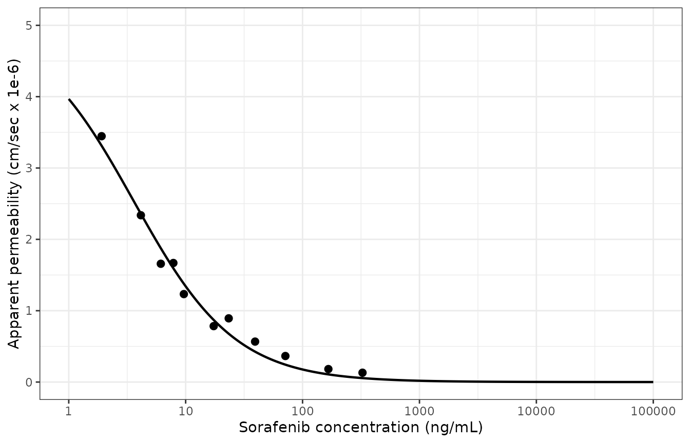
Replicates Figure 5 of Agarwal 2011: apparent B-to-A permeability of sorafenib across MDCKII-Bcrp1 monolayers. Points are the published observations recovered by digitisation; the line is the packaged model.
Structural checks
The defining property of Equation 2 is that km is, in
the authors’ words, “the concentration of sorafenib at which
half-maximal inhibition is seen” – so the curve must pass through
exactly emax / 2 at C = km. It must also
return emax at zero concentration and decay monotonically
to zero.
km <- exp(bcrp$theta[["lkm"]])
emax5 <- exp(bcrp$theta[["lemax"]])
chk5 <- solveStatic(bcrp, c(0, km, 1e9))
#> Warning: multi-subject simulation without without 'omega'

halfMax <- chk5$papp_ba[2]
tibble::tibble(
  Check = c("papp_ba at C = 0", "papp_ba at C = km", "emax / 2", "papp_ba at C = 1e9"),
  Value = c(chk5$papp_ba[1], halfMax, emax5 / 2, chk5$papp_ba[3])
) |>
knitr::kable(digits = 6)| Check | Value |
|---|---|
| papp_ba at C = 0 | 5.070 |
| papp_ba at C = km | 2.535 |
| emax / 2 | 2.535 |
| papp_ba at C = 1e9 | 0.000 |
Agreement with the published observations
cmp5 <- fig5_obs |>
  dplyr::mutate(
    papp_ba_pred = solveStatic(bcrp, conc_ngml)$papp_ba,
    abs_dev = papp_ba_pred - papp_ba_obs,
    pct_diff = 100 * abs_dev / papp_ba_obs
  )
#> Warning: There was 1 warning in `dplyr::mutate()`.
#> ℹ In argument: `papp_ba_pred = solveStatic(bcrp, conc_ngml)$papp_ba`.
#> Caused by warning:
#> ! multi-subject simulation without without 'omega'
knitr::kable(cmp5, digits = 3)| conc_ngml | papp_ba_obs | papp_ba_pred | abs_dev | pct_diff |
|---|---|---|---|---|
| 1.91 | 3.446 | 3.313 | -0.133 | -3.873 |
| 4.14 | 2.338 | 2.358 | 0.020 | 0.861 |
| 6.13 | 1.658 | 1.876 | 0.218 | 13.139 |
| 7.85 | 1.669 | 1.594 | -0.075 | -4.490 |
| 9.65 | 1.233 | 1.378 | 0.145 | 11.720 |
| 17.37 | 0.784 | 0.870 | 0.086 | 11.019 |
| 23.35 | 0.893 | 0.677 | -0.216 | -24.160 |
| 39.26 | 0.567 | 0.426 | -0.141 | -24.894 |
| 71.28 | 0.365 | 0.244 | -0.121 | -33.219 |
| 166.27 | 0.182 | 0.107 | -0.075 | -40.963 |
| 325.65 | 0.131 | 0.055 | -0.076 | -57.683 |
r2_5 <- 1 - sum(cmp5$abs_dev^2) / sum((cmp5$papp_ba_obs - mean(cmp5$papp_ba_obs))^2)
cat("R-squared:", round(r2_5, 4), "\n")
#> R-squared: 0.9814
Note that the relative deviation grows to nearly 60% at the
far right of the curve while the absolute deviation there is
under 0.08 x 1e-6 cm/s. That is an artefact of dividing by an
observation that is itself approaching zero, not a failure of the model,
so the tail is bounded on absolute deviation and only the informative
part of the curve (C <= 20 ng/mL, where the permeability is still a
substantial fraction of emax) is bounded on relative
deviation.
Model 2 – Inhibition of P-gp by sorafenib
The asymmetry the paper turns on: sorafenib inhibits P-gp but is not transported by it, and is a high-affinity BCRP substrate that does not inhibit BCRP. This model is therefore sorafenib acting as a perpetrator – raising the intracellular accumulation of the P-gp probe vinblastine.
Replicates Figure 6A of Agarwal 2011
grid6 <- 10^seq(log10(400), log10(1.2e5), length.out = 400)
pred6 <- solveStatic(pgp, grid6)
#> Warning: multi-subject simulation without without 'omega'

ggplot2::ggplot() +
  ggplot2::geom_line(
    data = pred6,
    ggplot2::aes(CP_SORAFENIB_NGML / 1000, vbl_accum), linewidth = 0.8
  ) +
  ggplot2::geom_point(
    data = fig6_obs,
    ggplot2::aes(conc_ugml, fold_obs), size = 2.2
  ) +
  ggplot2::scale_x_log10(breaks = c(1, 10, 100), labels = c("1", "10", "100")) +
  ggplot2::coord_cartesian(ylim = c(0, 14)) +
  ggplot2::labs(
    x = "Sorafenib concentration (ug/mL)",
    y = "Fold increase in vinblastine accumulation"
  ) +
  ggplot2::theme_bw()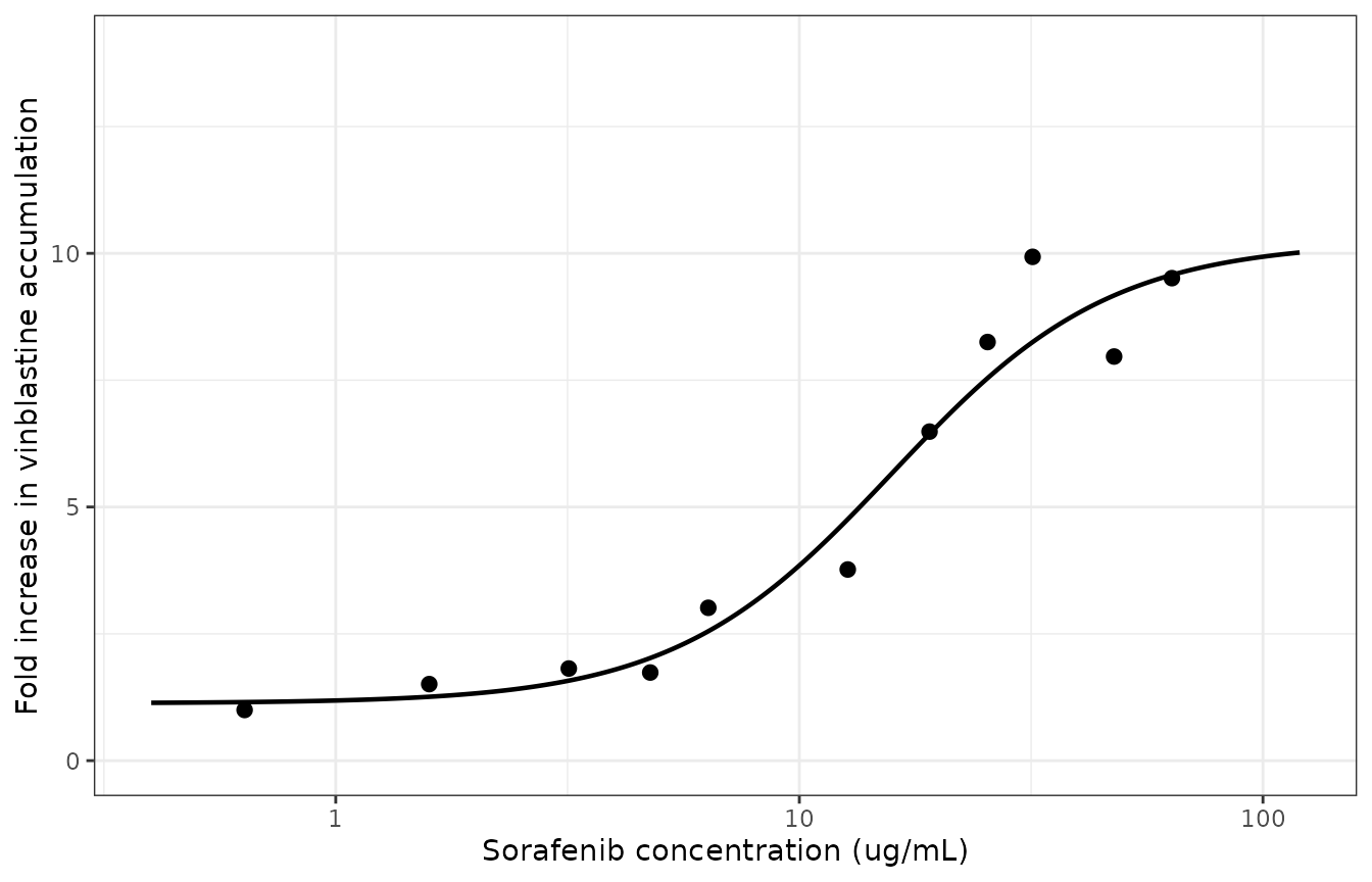
Replicates Figure 6A of Agarwal 2011: fold increase in intracellular vinblastine accumulation in MDCKII-MDR1 cells with increasing sorafenib. Points are the published observations recovered by digitisation; the line is the packaged model.
Structural checks
At C = ic50 a sigmoid Emax curve must sit exactly
halfway between its asymptotes, (e0 + emax) / 2. That
identity is what makes the published 15.9 ug/mL an IC50 rather than an
arbitrary scale parameter, and it is the single strongest check
available on this model.
ic50 <- exp(pgp$theta[["lic50"]])
e0 <- exp(pgp$theta[["le0"]])
emax6 <- exp(pgp$theta[["lemax"]])
hill <- exp(pgp$theta[["lhill"]])
chk6 <- solveStatic(pgp, c(0, ic50, 1e12))
#> Warning: multi-subject simulation without without 'omega'

tibble::tibble(
  Check = c("vbl_accum at C = 0", "e0", "vbl_accum at C = ic50", "(e0 + emax) / 2",
            "vbl_accum at C = 1e12", "emax"),
  Value = c(chk6$vbl_accum[1], e0, chk6$vbl_accum[2], (e0 + emax6) / 2,
            chk6$vbl_accum[3], emax6)
) |>
knitr::kable(digits = 6)| Check | Value |
|---|---|
| vbl_accum at C = 0 | 1.1300 |
| e0 | 1.1300 |
| vbl_accum at C = ic50 | 5.6805 |
| (e0 + emax) / 2 | 5.6805 |
| vbl_accum at C = 1e12 | 10.2310 |
| emax | 10.2310 |
stopifnot(
  abs(chk6$vbl_accum[1] - e0) < 1e-10,
  abs(chk6$vbl_accum[2] - (e0 + emax6) / 2) < 1e-10,
  abs(chk6$vbl_accum[3] - emax6) < 1e-6,
  all(diff(pred6$vbl_accum) > 0),
  # The Hill exponent is well above 1, so the curve is genuinely sigmoidal
  # rather than the hyperbolic (hill = 1) special case.
  hill > 1.5
)
Agreement with the published observations
cmp6 <- fig6_obs |>
  dplyr::mutate(
    fold_pred = solveStatic(pgp, conc_ngml)$vbl_accum,
    abs_dev = fold_pred - fold_obs,
    pct_diff = 100 * abs_dev / fold_obs
  ) |>
  dplyr::select(conc_ugml, fold_obs, fold_pred, abs_dev, pct_diff)
#> Warning: There was 1 warning in `dplyr::mutate()`.
#> ℹ In argument: `fold_pred = solveStatic(pgp, conc_ngml)$vbl_accum`.
#> Caused by warning:
#> ! multi-subject simulation without without 'omega'
knitr::kable(cmp6, digits = 3)| conc_ugml | fold_obs | fold_pred | abs_dev | pct_diff |
|---|---|---|---|---|
| 0.636 | 0.999 | 1.154 | 0.155 | 15.531 |
| 1.591 | 1.509 | 1.259 | -0.250 | -16.552 |
| 3.182 | 1.816 | 1.577 | -0.239 | -13.166 |
| 4.769 | 1.737 | 2.023 | 0.286 | 16.473 |
| 6.362 | 3.013 | 2.551 | -0.462 | -15.332 |
| 12.719 | 3.768 | 4.758 | 0.990 | 26.272 |
| 19.092 | 6.486 | 6.440 | -0.046 | -0.708 |
| 25.470 | 8.252 | 7.540 | -0.712 | -8.629 |
| 31.852 | 9.931 | 8.251 | -1.680 | -16.919 |
| 47.746 | 7.966 | 9.170 | 1.204 | 15.117 |
| 63.629 | 9.511 | 9.575 | 0.064 | 0.668 |
r2_6 <- 1 - sum(cmp6$abs_dev^2) / sum((cmp6$fold_obs - mean(cmp6$fold_obs))^2)
cat("R-squared:", round(r2_6, 4), "\n")
#> R-squared: 0.9486

stopifnot(
  r2_6 > 0.92,                          # measured 0.949
  max(abs(cmp6$abs_dev)) < 2.0,         # measured 1.68 fold
  max(abs(cmp6$pct_diff)) < 35          # measured 26.3
)
The scatter about the fitted curve is the authors’ own – the two points at 32 and 48 ug/mL straddle the curve by more than a fold in opposite directions in the published panel (their plotted SD bars are correspondingly wide, n = 4). The model reproduces the curve, which is what was extracted.
Clinical relevance of the IC50
# The authors note (Discussion) that sorafenib plasma concentrations on the
# accepted 100-400 mg b.i.d. regimen are 1-15 uM. The paper's own dual-unit
# report (15.9 ug/mL = 25 uM) implies 636 g/mol -- sorafenib tosylate, the
# salt purchased in Methods -- NOT the 464.8 g/mol free base.
mw_tosylate <- 15900 / 25    # ng/mL per uM, from the paper's own conversion
clinical <- solveStatic(pgp, c(1, 5, 15) * mw_tosylate)
#> Warning: multi-subject simulation without without 'omega'
tibble::tibble(
  `Plasma sorafenib (uM)` = c(1, 5, 15),
  `Predicted fold increase in P-gp substrate accumulation` = clinical$vbl_accum
) |>
knitr::kable(digits = 2)| Plasma sorafenib (uM) | Predicted fold increase in P-gp substrate accumulation |
|---|---|
| 1 | 1.15 |
| 5 | 1.58 |
| 15 | 3.68 |
stopifnot(
  # The clinical range reaches the foot of the curve but not its plateau:
  # at 15 uM the model predicts a real but sub-maximal effect.
  clinical$vbl_accum[1] < 1.5,
  clinical$vbl_accum[3] > 2, clinical$vbl_accum[3] < emax6 / 2
)
At the top of the clinical range sorafenib is predicted to raise the tissue accumulation of a P-gp substrate roughly 3.7-fold – consistent with the authors’ warning that sorafenib “may alter tissue pharmacokinetics of concurrently administered drugs if the coadministered drug is a substrate for P-gp”.
In vivo results (context; not modelled)
The paper’s mouse work was analysed by noncompartmental analysis only – no compartmental or physiological model was fitted to the in vivo data – so there is no third model file. The key results are reproduced here as context for the two in vitro models, and because the in vivo / in vitro discordance is the paper’s main scientific point.
| Parameter | Plasma | Brain |
|---|---|---|
| Terminal rate constant (1/h) | 0.42 | 0.73 |
| Half-life (h) | 1.6 | 0.9 |
| Clearance (mL/min/kg) | 5.8 | – |
| Volume of distribution (mL/kg) | 840 | – |
| AUC 0-inf (mg*min/mL) | 1.6 | 0.11 |
| AUC brain / AUC plasma | 0.06 |
| Genotype | Plasma Css (ug/mL) | Brain Css (ug/g) | Brain-to-plasma ratio |
|---|---|---|---|
| FVB (wild-type) | 2.5 +/- 0.16 | 0.32 +/- 0.18 | 0.094 +/- 0.007 |
| Bcrp1 (-/-) | 1.5 +/- 0.42 | 0.51 +/- 0.074 | 0.36 +/- 0.056 |
| Mdr1a/b (-/-) | 3.07 +/- 0.91 | 0.34 +/- 0.16 | 0.11 +/- 0.021 |
| Mdr1a/b (-/-) Bcrp1 (-/-) | 1.9 +/- 0.17 | 1.7 +/- 0.69 | 0.91 +/- 0.29 |
The brain-to-plasma ratio rises about 4-fold when BCRP alone is knocked out but about 10-fold when both transporters are absent, even though knocking out P-gp alone changes nothing. That is the cooperation the authors describe: BCRP is dominant for sorafenib, but P-gp still restricts brain entry once BCRP is gone.
# Consistency check internal to the paper, not a model prediction: the
# equilibrium distribution coefficient from the IV study (AUCbrain/AUCplasma)
# should agree with the steady-state brain-to-plasma ratio in wild-type mice.
iv_ratio <- 0.06        # Table 1
ss_ratio <- 0.094       # Table 2, wild-type
stopifnot(abs(iv_ratio - ss_ratio) < 0.05)
Assumptions and deviations
Values not printed in the source
emax (BCRP), and e0, emax and
hill (P-gp) are not reported anywhere in
the article – not in the text, not in a table, not in a figure panel
annotation. They were recovered by digitising the published figures, as
permitted for figure-only parameters. The two km /
ic50 values that are printed were held fixed at
their published values throughout; figure-fitting filled gaps and never
overrode a printed number.
The P-gp digitisation self-validates: refitting the
traced Figure 6A curve with all four parameters free returns
ic50 = 15.48 ug/mL against the printed 15.9 +/- 3.8 ug/mL,
a 2.7% recovery error, which bounds the accuracy of the whole trace. The
BCRP digitisation validates the same way: refitting Equation 2 to the
Figure 5 observations with both parameters free returns km
= 3.13 ng/mL (SE 0.41) against the printed 3.6 +/- 0.78 ng/mL, well
within one standard error.
e0 is not exactly 1
Methods Equation 3 glosses E0 as “the accumulation of
probe in the absence of sorafenib normalized to unity”, which reads as
E0 = 1 exactly. The authors’ own plotted curve, however,
has a left asymptote of 1.130. The sentence describes how the
data were normalised, not a constraint on the fitted
parameter, so e0 is encoded at the digitised 1.130 – which
reproduces the published figure, where 1.000 does not. Users who prefer
the literal reading can set le0 <- log(1) and refit;
that variant gives emax about 10.25 and hill
about 2.02.
Errata – three demonstrable errors in the Figure 5 caption
The Figure 5 caption contradicts the Methods, the Results, and the figure’s own panel on three separate points. This file follows Methods Equation 2 and the Results/panel estimate throughout.
| Figure 5 caption says | Correct value | Where the correct value appears |
|---|---|---|
| affinity “determined to be 5 nM” | 5.5 nM | Results text and the Figure 5 panel |
| “A sigmoid inhibitory Emax model” | non-sigmoid hyperbolic; no Hill exponent | Methods Eq 2 and the equation printed in the panel |
| range “(0.001 nM to 80 nM)” | 2 ng/mL to 30 ug/mL | Methods, and the panel’s own x-axis (1 to 1e5 ng/mL) |
The published Figure 5 curve is not internally consistent
The dashed “Model Predicted” trace in Figure 5 cannot be reconciled
with Equation 2 at the printed km = 3.6 ng/mL. Its
half-maximal point implies emax = 4.94 while its value at C
= 1 ng/mL implies emax = 6.15, and refitting the traced
curve with km free returns km = 2.27 – well
below the printed value. The observed points, by
contrast, are consistent with the printed km, so
emax was fitted to the observations rather than to the
drawn curve. Fitting to the curve instead would give emax =
5.34, so the choice moves emax by about 5%; the two routes
bracket it at roughly 5.1-5.3 x 1e-6 cm/s. No such inconsistency exists
in Figure 6A.
Molecular weight used for mass / molar conversion
The paper reports both potencies in dual units: 3.6 ng/mL = 5.5 nM (implying about 655 g/mol) and 15.9 ug/mL = 25 uM (implying 636 g/mol). Neither is the sorafenib free base at 464.8 g/mol; both are consistent with sorafenib tosylate, 637.0 g/mol, the salt purchased in Methods. Anyone converting the packaged ng/mL values to molar units with the free-base weight will disagree with every printed molar figure in the paper by about 37%.
No variability components
Neither model carries inter-individual variability or residual error.
Each is a single fitted concentration-response curve from one
cell-culture experiment; the source reports point estimates with
standard errors of the estimate and replicate SDs on the plotted means,
but no variance components. Per the standing policy on unreported
residual error, addSd is fixed at 0 so each model returns
its deterministic curve. Do not read the plotted SD bars in Figures 5
and 6A as an IIV or RUV estimate – they are replicate spread (n = 3 and
n = 4 wells), not a fitted variance.
Two new canonical observation names
Neither endpoint could reuse an existing canonical: Cc
would be wrong because neither is a drug concentration
(papp_ba is an apparent permeability in cm/sec,
vbl_accum is a dimensionless fold change in the
accumulation of a different drug, vinblastine), and a search of
the 658-entry observation register for permeability / flux / efflux /
accumulation / fold / transport / uptake turned up nothing either name
could alias. Both names were therefore ratified by the maintainers
before this model file was added, and are registered in
inst/references/compartment-names.md:
-
papp_ba– apparent basolateral-to-apical permeability, withpapp_abreserved for the opposite direction. The direction is part of the name rather than a note in the entry because directional flux is the entire point of a Transwell assay: this paper reports both directions (Figure 3), so a barepappwould silently conflate two different measured quantities the first time an A-to-B model were added. The qualified form also avoids a collision withpapp, which already exists in the registry as anini()parameter name for apparent permeability in the threeGranda_2024_*_pbpkmodels. -
vbl_accum– fold increase in intracellular vinblastine accumulation, named for the specific probe in the same wayherg_inhnames a specific channel’s tail-current block. A genericprobeAccumFoldwould need the probe recorded out-of-band to be interpretable; this paper alone uses three different probes (vinblastine for P-gp, prazosin and mitoxantrone for BCRP).
Both names are expected to be reused: the same directional-Transwell and probe-accumulation assay design recurs across the sibling Elmquist-lab TKI papers this one cites (gefitinib, dasatinib, erlotinib, lapatinib, imatinib).
Not extracted from this paper
- The in vivo mouse PK (single 10 mg/kg IV dose; 48 h intraperitoneal infusions in four genotypes; the elacridar interaction study) was analysed by noncompartmental analysis only. There is no fitted compartmental or physiological model to extract, so the results appear above as context only.
- A BCRP inhibition curve does not exist: sorafenib did not increase accumulation of either prazosin or mitoxantrone in the Bcrp1 transfects (Figure 6B), so no model was fitted to that panel. The authors infer that sorafenib binds BCRP at a site not overlapping those probes.
-
The Papp calculation itself
(
Papp = (dQ/dt) / (A * C0), monolayer area A = 4.67 cm^2, Methods Equation 1) is a data-reduction step applied before either model is fitted, not part of a model, so it is not encoded.