Atezolizumab exposure-response in high tumour mutational burden (Shemesh 2020) • nlmixr2lib

Model and source

Citation: Shemesh CS, Chan P, Legrand FA, et al. Pan-cancer population pharmacokinetics and exposure-safety and -efficacy analyses of atezolizumab in patients with high tumor mutational burden. Pharmacol Res Perspect. 2020;8(6):e00685.
Article: https://doi.org/10.1002/prp2.685 (open access; Supporting Information file s001 holds Tables S1-S3 and Figures S1-S7)

Shemesh 2020 pooled 986 patients with tissue tumour mutational burden (tTMB) data from seven single-agent atezolizumab trials and asked whether patients with high tTMB (>= 16 mutations/Mb) have different exposure, and whether exposure predicts efficacy or safety in that group. PK was not re-estimated: the authors applied the phase I population PK model of Stroh et al. (Clin Pharmacol Ther 2017;102:305-312) with Bayesian post hoc estimation (MAXEVAL = 0) and derived Cycle-1 AUC, C_max and C_min for every patient. They then fitted logistic regressions of three endpoints on each exposure metric in the tTMB-high subgroup:

models <- tibble::tribble(
  ~Model,                                     ~Endpoint,                      ~Exposure,       ~Figure,
  "Shemesh_2020_atezolizumab_orr_auc",        "Objective response",           "Cycle-1 AUC",   "3A",
  "Shemesh_2020_atezolizumab_orr_ctrough",    "Objective response",           "Cycle-1 Cmin",  "3B",
  "Shemesh_2020_atezolizumab_orr_cmax",       "Objective response",           "Cycle-1 Cmax",  "S6A",
  "Shemesh_2020_atezolizumab_aeg34_auc",      "Grade 3/4 adverse event",      "Cycle-1 AUC",   "3C",
  "Shemesh_2020_atezolizumab_aeg34_ctrough",  "Grade 3/4 adverse event",      "Cycle-1 Cmin",  "S6B",
  "Shemesh_2020_atezolizumab_aeg34_cmax",     "Grade 3/4 adverse event",      "Cycle-1 Cmax",  "S6C",
  "Shemesh_2020_atezolizumab_aesi_auc",       "Any-grade AESI",               "Cycle-1 AUC",   "3D",
  "Shemesh_2020_atezolizumab_aesi_ctrough",   "Any-grade AESI",               "Cycle-1 Cmin",  "S6D",
  "Shemesh_2020_atezolizumab_aesi_cmax",      "Any-grade AESI",               "Cycle-1 Cmax",  "S6E"
)
knitr::kable(models, caption = "The nine packaged exposure-response models.")

The nine packaged exposure-response models.
Model	Endpoint	Exposure	Figure
Shemesh_2020_atezolizumab_orr_auc	Objective response	Cycle-1 AUC	3A
Shemesh_2020_atezolizumab_orr_ctrough	Objective response	Cycle-1 Cmin	3B
Shemesh_2020_atezolizumab_orr_cmax	Objective response	Cycle-1 Cmax	S6A
Shemesh_2020_atezolizumab_aeg34_auc	Grade 3/4 adverse event	Cycle-1 AUC	3C
Shemesh_2020_atezolizumab_aeg34_ctrough	Grade 3/4 adverse event	Cycle-1 Cmin	S6B
Shemesh_2020_atezolizumab_aeg34_cmax	Grade 3/4 adverse event	Cycle-1 Cmax	S6C
Shemesh_2020_atezolizumab_aesi_auc	Any-grade AESI	Cycle-1 AUC	3D
Shemesh_2020_atezolizumab_aesi_ctrough	Any-grade AESI	Cycle-1 Cmin	S6D
Shemesh_2020_atezolizumab_aesi_cmax	Any-grade AESI	Cycle-1 Cmax	S6E

Every one of the nine relationships is non-significant; that flat exposure-response is the paper’s conclusion and what supports a single 1200 mg every-3-week regimen in a tumour-agnostic high-tTMB population. The PK model itself is not packaged again here: the parameter set Shemesh 2020 prints is the fixed intravenous disposition layer of Chan_2025_atezolizumab (checked below), and that model is used to generate the exposures this vignette feeds into the exposure-response models.

The paper also plots exploratory tTMB-response curves (Figure S7). Those are not packaged; see “Assumptions and deviations”.

Population

The exposure-response analyses use the tTMB-high patients with exposure data: 171 for objective response and any-grade adverse events of special interest (AESIs), and 167 for grade 3/4 adverse events. They come from OAK, POPLAR, BIRCH, FIR, IMvigor210, IMvigor211 and PCD4989g (Table S1). About 94% received 1200 mg IV every 3 weeks; some PCD4989g patients received 10, 15 or 20 mg/kg. The tTMB-high column of Table 1 (n = 175) gives:

median age 65 (37-89) years
median body weight 75 (35.4-149) kg
27.4% female and 82.9% White
median albumin 39 g/L and median baseline sum of longest diameters (SLD) 58 mm
29.3% ADA-positive

The largest tumour groups were NSCLC (83) and urothelial carcinoma (70), followed by melanoma (12) and at least five other types (Table S2). The same summary is stored in each model’s population metadata, for example readModelDb("Shemesh_2020_atezolizumab_orr_auc")()$population.

Source trace

Shemesh 2020 prints no logistic-regression coefficients anywhere in the article or supplement, only exploratory P values and the fitted curves. Every coefficient below was therefore recovered from the drawing:

Figure 3 (main article) is embedded in the PDF as vector graphics. The maintainers read the fitted curve’s end points exactly from the drawing coordinates, calibrated against the axis tick marks, and solved the two logistic coefficients from them.
Figure S6 (supplement) is a raster image. The fitted curve was traced column by column (about 160-190 points per panel) and fitted in probability space. The residual SD was 0.001-0.003 on the probability scale, which is at or below one pixel.

The functional form was not assumed. On the logit scale, a line in the untransformed exposure reproduces every panel’s curvature. A line in log exposure does not: its logit RMSE was 5-35 times larger on the S6 traces, and it misses the two interior points of the Figure 3D Bezier curve by about 0.09 in probability (checked below).

coefs <- tibble::tribble(
  ~Model,                                    ~Intercept, ~Slope,   ~`Slope unit`,        ~`Printed P`, ~Source,
  "Shemesh_2020_atezolizumab_orr_auc",       -0.5972,    -0.09243, "per 1000 ug*day/mL", ".751",       "Figure 3A (vector)",
  "Shemesh_2020_atezolizumab_orr_ctrough",   -0.8660,     0,       "per 10 ug/mL",       ".998",       "Figure 3B (vector; drawn exactly flat)",
  "Shemesh_2020_atezolizumab_orr_cmax",       0.4876,    -0.3537,  "per 100 ug/mL",      ".1072",      "Figure S6A (raster)",
  "Shemesh_2020_atezolizumab_aeg34_auc",      0.4644,    -0.06491, "per 1000 ug*day/mL", ".812",       "Figure 3C (vector)",
  "Shemesh_2020_atezolizumab_aeg34_ctrough",  0.9521,    -0.0902,  "per 10 ug/mL",       ".2217",      "Figure S6B (raster)",
  "Shemesh_2020_atezolizumab_aeg34_cmax",    -0.1414,     0.1038,  "per 100 ug/mL",      ".5714",      "Figure S6C (raster)",
  "Shemesh_2020_atezolizumab_aesi_auc",      -1.7908,     0.2994,  "per 1000 ug*day/mL", ".280",       "Figure 3D (vector)",
  "Shemesh_2020_atezolizumab_aesi_ctrough",  -0.7491,     0.0468,  "per 10 ug/mL",       ".5248",      "Figure S6D (raster)",
  "Shemesh_2020_atezolizumab_aesi_cmax",     -0.1891,    -0.0547,  "per 100 ug/mL",      ".7715",      "Figure S6E (raster)"
)
knitr::kable(coefs, caption = "Logistic coefficients: logit(p) = Intercept + Slope * exposure / scale. P values are printed in Results 3.4-3.5 (Figure 3) and on the Figure S6 panels.")

Logistic coefficients: logit(p) = Intercept + Slope * exposure / scale. P values are printed in Results 3.4-3.5 (Figure 3) and on the Figure S6 panels.
Model	Intercept	Slope	Slope unit	Printed P	Source
Shemesh_2020_atezolizumab_orr_auc	-0.5972	-0.09243	per 1000 ug*day/mL	.751	Figure 3A (vector)
Shemesh_2020_atezolizumab_orr_ctrough	-0.8660	0.00000	per 10 ug/mL	.998	Figure 3B (vector; drawn exactly flat)
Shemesh_2020_atezolizumab_orr_cmax	0.4876	-0.35370	per 100 ug/mL	.1072	Figure S6A (raster)
Shemesh_2020_atezolizumab_aeg34_auc	0.4644	-0.06491	per 1000 ug*day/mL	.812	Figure 3C (vector)
Shemesh_2020_atezolizumab_aeg34_ctrough	0.9521	-0.09020	per 10 ug/mL	.2217	Figure S6B (raster)
Shemesh_2020_atezolizumab_aeg34_cmax	-0.1414	0.10380	per 100 ug/mL	.5714	Figure S6C (raster)
Shemesh_2020_atezolizumab_aesi_auc	-1.7908	0.29940	per 1000 ug*day/mL	.280	Figure 3D (vector)
Shemesh_2020_atezolizumab_aesi_ctrough	-0.7491	0.04680	per 10 ug/mL	.5248	Figure S6D (raster)
Shemesh_2020_atezolizumab_aesi_cmax	-0.1891	-0.05470	per 100 ug/mL	.7715	Figure S6E (raster)


# Confirm that every packaged file carries exactly these values.
iniOf <- function(m) {
  ui <- rxode2::rxode(readModelDb(m))
  th <- ui$theta
  th[!grepl("^addSd_", names(th))]
}
packaged <- lapply(coefs$Model, iniOf)
stopifnot(
  all(vapply(packaged, length, integer(1)) == 2L),
  isTRUE(all.equal(unname(vapply(packaged, function(x) x[["logit_ref"]], numeric(1))), coefs$Intercept)),
  isTRUE(all.equal(unname(vapply(packaged, function(x) x[[setdiff(names(x), "logit_ref")]], numeric(1))), coefs$Slope))
)

The exposure metrics are defined in Methods 2.4. C_max is the end-of-infusion value on day 1 of cycle 1. C_min is the day-1 cycle-2 pre-dose value, which is the day-21 trough after one dose, so it is carried by the CTROUGH canonical. AUC is the Cycle-1 AUC over the 21-day cycle (AUC_ATEZO). All three are model-predicted total serum concentrations.

The PK equations match the packaged intravenous layer

Methods 2.4 prints the typical-value equations of the Stroh 2017 model used to derive the exposures:

CL = 0.200 (ALB/40)^-1.12 (BWT/77)^0.808 (tumour burden/63)^0.125, times 1.159 if ADA-positive
V1 = 3.28 (BWT/77)^0.559 (ALB/40)^-0.350, times 0.871 if female
V2 = 3.63, times 0.728 if female

Chan_2025_atezolizumab carries the same model as its fixed intravenous layer. Its categorical effects are written as (1 + theta), so 1.159, 0.871 and 0.728 correspond to 0.159, -0.129 and -0.272.

pk <- rxode2::rxode(readModelDb("Chan_2025_atezolizumab"))$theta
#> ℹ parameter labels from comments will be replaced by 'label()'
shemeshPrinted <- c(
  lcl = log(0.200), e_alb_cl = -1.12, e_wt_cl = 0.808, e_tumsz_cl = 0.125,
  e_ada_cl = 1.159 - 1, lvc = log(3.28), e_wt_vc = 0.559, e_alb_vc = -0.350,
  e_sexf_vc = 0.871 - 1, lvp = log(3.63), e_sexf_vp = 0.728 - 1
)
# Same parameter set, so the agreement is exact to the printed digits.
stopifnot(isTRUE(all.equal(unname(pk[names(shemeshPrinted)]), unname(shemeshPrinted), tolerance = 1e-12)))
knitr::kable(
  data.frame(parameter = names(shemeshPrinted),
             `Shemesh 2020 Methods` = signif(unname(shemeshPrinted), 4),
             `Chan_2025_atezolizumab` = signif(unname(pk[names(shemeshPrinted)]), 4),
             check.names = FALSE),
  caption = "Every printed typical-value term matches the packaged intravenous layer. Q (0.546 L/day), the IIV block and the residual error are not printed by Shemesh 2020 and are taken from the packaged model."
)

Every printed typical-value term matches the packaged intravenous layer. Q (0.546 L/day), the IIV block and the residual error are not printed by Shemesh 2020 and are taken from the packaged model.
parameter	Shemesh 2020 Methods	Chan_2025_atezolizumab
lcl	-1.609	-1.609
e_alb_cl	-1.120	-1.120
e_wt_cl	0.808	0.808
e_tumsz_cl	0.125	0.125
e_ada_cl	0.159	0.159
lvc	1.188	1.188
e_wt_vc	0.559	0.559
e_alb_vc	-0.350	-0.350
e_sexf_vc	-0.129	-0.129
lvp	1.289	1.289
e_sexf_vp	-0.272	-0.272

Virtual cohort

The tTMB-high cohort is rebuilt from the Table 1 medians and ranges. The distributional shapes (log-normal weight and SLD, normal albumin, each truncated to the printed range) are assumptions, because Table 1 reports only medians and ranges. Hemoglobin affects only subcutaneous bioavailability in Chan_2025_atezolizumab and is irrelevant to IV dosing; it is set to that model’s reference value.

rxode2::rxSetSeed(20201124)
nSub <- 171

truncNorm <- function(n, mu, sd, lo, hi) {
  x <- numeric(0)
  while (length(x) < n) {
    y <- stats::rnorm(n, mu, sd)
    x <- c(x, y[y >= lo & y <= hi])
  }
  x[seq_len(n)]
}

cohort <- data.frame(
  id = seq_len(nSub),
  WT = exp(truncNorm(nSub, log(75), 0.22, log(35.4), log(149))),
  ALB = truncNorm(nSub, 39, 4.5, 20, 49),
  TUMSZ = exp(truncNorm(nSub, log(58), 0.75, log(11.1), log(309))),
  ADA_POS = stats::rbinom(nSub, 1, 0.293),
  SEXF = stats::rbinom(nSub, 1, 0.274),
  HGB = 123
)
summary(cohort[, c("WT", "ALB", "TUMSZ")])
#>        WT              ALB            TUMSZ       
#>  Min.   : 42.21   Min.   :27.99   Min.   : 11.31  
#>  1st Qu.: 66.56   1st Qu.:35.46   1st Qu.: 33.11  
#>  Median : 76.16   Median :39.34   Median : 52.34  
#>  Mean   : 77.41   Mean   :39.32   Mean   : 67.22  
#>  3rd Qu.: 85.85   3rd Qu.:42.89   3rd Qu.: 87.61  
#>  Max.   :137.51   Max.   :48.95   Max.   :294.66

Simulation of Cycle-1 exposure

One 1200 mg dose is given by 60-minute IV infusion into central, with dense sampling over the first cycle. The window closes at day 20.999 so that the trough is not contaminated by a cycle-2 dose.

obsTimes <- sort(unique(c(seq(0, 0.25, by = 1 / 96), seq(0.25, 2, by = 0.25),
                          seq(2.5, 20.5, by = 0.5), 20.999)))
events <- bind_rows(
  data.frame(id = cohort$id, time = 0, amt = 1200, rate = 1200 * 24,
             evid = 1L, cmt = "central"),
  tidyr::expand_grid(id = cohort$id, time = obsTimes) |>
    mutate(amt = NA_real_, rate = NA_real_, evid = 0L, cmt = "central")
) |>
  arrange(id, time, desc(evid)) |>
  left_join(cohort, by = "id")

sim <- rxode2::rxSolve(rxode2::rxode(readModelDb("Chan_2025_atezolizumab")),
                       events, returnType = "data.frame") |>
  mutate(treatment = "1200 mg IV, tTMB-high")
#> ℹ parameter labels from comments will be replaced by 'label()'

sim |>
  group_by(time) |>
  summarise(median = median(Cc), lo = quantile(Cc, 0.05), hi = quantile(Cc, 0.95),
            .groups = "drop") |>
  ggplot(aes(time, median)) +
  geom_ribbon(aes(ymin = lo, ymax = hi), alpha = 0.2) +
  geom_line() +
  scale_y_log10() +
  labs(x = "Time (day)", y = "Atezolizumab serum concentration (ug/mL)",
       title = "Simulated Cycle-1 profiles, virtual tTMB-high cohort",
       subtitle = "Median with 5th-95th percentile band") +
  theme_bw()
#> Warning in scale_y_log10(): log-10 transformation introduced infinite values.
#> log-10 transformation introduced infinite values.
#> log-10 transformation introduced infinite values.
#> log-10 transformation introduced infinite values.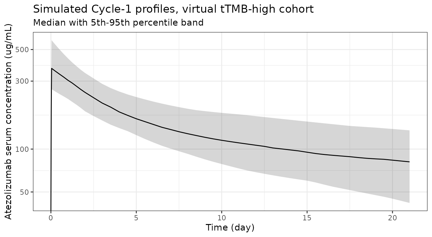

PKNCA validation

# rxSolve returns only the observation grid, so the concentration frame needs
# no evid filter; the filter is !is.na(Cc) alone so the time-zero row survives.
concData <- sim |>
  filter(!is.na(Cc)) |>
  select(id, time, Cc, treatment)
doseData <- data.frame(id = cohort$id, time = 0, amt = 1200,
                       treatment = "1200 mg IV, tTMB-high")
stopifnot(all(tapply(concData$time, concData$id, min) == 0))

concObj <- PKNCA::PKNCAconc(concData, Cc ~ time | treatment + id,
                            concu = "ug/mL", timeu = "day")
doseObj <- PKNCA::PKNCAdose(doseData, amt ~ time | treatment + id, doseu = "mg")
intervals <- data.frame(start = 0, end = 20.999, cmax = TRUE, auclast = TRUE)
ncaRes <- PKNCA::pk.nca(PKNCA::PKNCAdata(concObj, doseObj, intervals = intervals))

ncaIndiv <- as.data.frame(ncaRes) |>
  filter(PPTESTCD %in% c("cmax", "auclast")) |>
  select(id, PPTESTCD, PPORRES) |>
  tidyr::pivot_wider(names_from = PPTESTCD, values_from = PPORRES)

# The day-21 trough is read off the solve rather than through PKNCA, whose
# ctrough needs an interval ending on a dose record.
exposure <- sim |>
  filter(abs(time - 20.999) < 1e-9) |>
  select(id, ctrough = Cc) |>
  inner_join(ncaIndiv, by = "id") |>
  mutate(treatment = "1200 mg IV, tTMB-high")
stopifnot(nrow(exposure) == nSub, !anyNA(exposure))

geoMean <- function(x) exp(mean(log(x)))
simulatedSummary <- exposure |>
  group_by(treatment) |>
  summarise(cmax = geoMean(cmax), ctrough = geoMean(ctrough),
            auclast = geoMean(auclast), .groups = "drop") |>
  tidyr::pivot_longer(-treatment, names_to = "PPTESTCD", values_to = "PPORRES")

Comparison against the published exposure metrics

Table 2 of Shemesh 2020 reports geometric means of the post hoc Cycle-1 exposures in the 171 tTMB-high patients.

published <- tibble::tribble(
  ~treatment,              ~PPTESTCD, ~PPORRES,
  "1200 mg IV, tTMB-high", "cmax",    367,
  "1200 mg IV, tTMB-high", "ctrough", 63.2,
  "1200 mg IV, tTMB-high", "auclast", 2722
)
cmp <- nlmixr2lib::ncaComparisonTable(
  simulated = simulatedSummary,
  reference = published,
  by = "treatment",
  units = c(cmax = "ug/mL", ctrough = "ug/mL", auclast = "ug*day/mL"),
  tolerance_pct = 20
)
cmp |>
  dplyr::rename("Treatment" = treatment) |>
  knitr::kable(caption = paste(
    "Simulated Cycle-1 geometric means versus Shemesh 2020 Table 2 (tTMB-high).",
    "* differs from the published value by more than 20%."
  ))

Simulated Cycle-1 geometric means versus Shemesh 2020 Table 2 (tTMB-high). * differs from the published value by more than 20%.
NCA parameter	Treatment	Reference	Simulated	% diff
Cmax (ug/mL)	1200 mg IV, tTMB-high	367	381	+3.9%
AUClast (ug*day/mL)	1200 mg IV, tTMB-high	2720	2940	+8.2%
Ctrough (ug/mL)	1200 mg IV, tTMB-high	63.2	78.1	+23.5%*


pctDiff <- inner_join(
  dplyr::rename(published, reference = PPORRES),
  dplyr::rename(simulatedSummary, simulated = PPORRES),
  by = c("treatment", "PPTESTCD")
) |>
  mutate(pct = 100 * (simulated - reference) / reference)
stopifnot(
  nrow(pctDiff) == 3L,
  # Cmax is dose / Vc to first order and depends only on the tightly
  # distributed weight, albumin and sex covariates, so it is the sharpest
  # check on the transcribed volumes.
  abs(pctDiff$pct[pctDiff$PPTESTCD == "cmax"]) < 10,
  # Centre of the three metrics. A mis-transcribed clearance or dose moves
  # AUC and the trough by tens of percent.
  abs(median(pctDiff$pct)) < 15,
  # The trough runs about 17-24% high across cohort seeds (see below); the
  # bound leaves headroom for cross-build RNG differences.
  max(abs(pctDiff$pct)) < 35
)

C_max reproduces within about 5% and AUC within about 10%. The simulated trough is starred: it sits about 20% above the published geometric mean. It fell between +17% and +24% across repeated cohort seeds, so the offset is systematic, not sampling noise. Table 2 reports a 200% CV for C_min against 30% for C_max, so the published exposures have a long low-concentration tail from a few patients with very high clearance. The paper notes that these “large %CV associated with C_min are related to the low exposure levels observed in a small number of patients”. A log-normal IIV model with a covariate cohort rebuilt from medians does not produce that tail. The tail pulls the observed geometric mean down, and it matters most for the trough, which is the metric most sensitive to clearance. The PK parameters are the paper’s own and were not adjusted.

Exposure-response

The digitised curves

The first check comes from the one panel whose fitted curve is drawn as a Bezier curve rather than a straight segment, Figure 3D. Its two interior junction points were not used to solve the coefficients (only the end points were), so they are an out-of-sample check on both the coefficients and the linear-in-AUC form.

# These models are purely algebraic: no ODE, no dose, no time dimension. A
# covariate grid is swept along a dummy time axis for a single subject.
solveStatic <- function(modelName, covs) {
  n <- max(vapply(covs, length, integer(1)))
  ev <- data.frame(id = 1L, time = seq_len(n), amt = 0, evid = 0L)
  for (nm in names(covs)) ev[[nm]] <- rep_len(covs[[nm]], n)
  s <- as.data.frame(rxode2::rxSolve(
    rxode2::zeroRe(rxode2::rxode(readModelDb(modelName))),
    events = ev, returnType = "data.frame"
  ))
  stopifnot(nrow(s) == n)
  s
}

interior <- data.frame(AUC_ATEZO = c(2081.9, 3871.6), digitised = c(0.2359, 0.3461))
interior$model <- solveStatic("Shemesh_2020_atezolizumab_aesi_auc",
                              list(AUC_ATEZO = interior$AUC_ATEZO))$prob_aesi
#> Warning: No omega parameters in the model
# The alternative log-AUC reading, fitted through the same two end points.
b1log <- (qlogis(0.4366) - qlogis(0.1539)) / log(5129.7 / 289.7)
interior$logAUC_form <- plogis(qlogis(0.1539) + b1log * log(interior$AUC_ATEZO / 289.7))
knitr::kable(interior, digits = 4,
             caption = "Figure 3D interior points versus the packaged model and the rejected log-AUC form.")

Figure 3D interior points versus the packaged model and the rejected log-AUC form.
AUC_ATEZO	digitised	model	logAUC_form
2081.9	0.2359	0.2373	0.3297
3871.6	0.3461	0.3471	0.4021

stopifnot(
  # Deterministic (no cohort, no RNG): the bound is the drawing resolution.
  all(abs(interior$model - interior$digitised) < 0.005),
  all(abs(interior$logAUC_form - interior$digitised) > 0.05)
)

Agreement with the plotted quartile proportions

Each panel also plots the observed proportion with the event in each exposure quartile, placed at the bin’s median exposure. These points were digitised in the same way (Figure 3 exactly; Figure S6 by pixel centroid). The quartile bins hold equal numbers of patients. So the mean of the four proportions is the observed incidence, and for a fitted logistic regression it must match the mean fitted probability. That is the maximum-likelihood score identity, a property of the fit rather than of the drawing.

bins <- tibble::tribble(
  ~Model,                                    ~exposure, ~observed,
  "Shemesh_2020_atezolizumab_orr_auc",        2349.1,   0.3022,
  "Shemesh_2020_atezolizumab_orr_auc",        2693.2,   0.2791,
  "Shemesh_2020_atezolizumab_orr_auc",        3055.0,   0.3561,
  "Shemesh_2020_atezolizumab_orr_auc",        3657.7,   0.2564,
  "Shemesh_2020_atezolizumab_orr_ctrough",      54.2,   0.2535,
  "Shemesh_2020_atezolizumab_orr_ctrough",      66.5,   0.3468,
  "Shemesh_2020_atezolizumab_orr_ctrough",      79.1,   0.3072,
  "Shemesh_2020_atezolizumab_orr_ctrough",      95.9,   0.2762,
  "Shemesh_2020_atezolizumab_orr_cmax",        287.2,   0.327,
  "Shemesh_2020_atezolizumab_orr_cmax",        349.3,   0.374,
  "Shemesh_2020_atezolizumab_orr_cmax",        408.7,   0.278,
  "Shemesh_2020_atezolizumab_orr_cmax",        489.9,   0.213,
  "Shemesh_2020_atezolizumab_aeg34_auc",      2374.0,   0.5405,
  "Shemesh_2020_atezolizumab_aeg34_auc",      2700.3,   0.5682,
  "Shemesh_2020_atezolizumab_aeg34_auc",      3072.2,   0.6554,
  "Shemesh_2020_atezolizumab_aeg34_auc",      3662.9,   0.4976,
  "Shemesh_2020_atezolizumab_aeg34_ctrough",    49.8,   0.667,
  "Shemesh_2020_atezolizumab_aeg34_ctrough",    68.2,   0.480,
  "Shemesh_2020_atezolizumab_aeg34_ctrough",    82.7,   0.596,
  "Shemesh_2020_atezolizumab_aeg34_ctrough",   101.8,   0.541,
  "Shemesh_2020_atezolizumab_aeg34_cmax",      293.7,   0.493,
  "Shemesh_2020_atezolizumab_aeg34_cmax",      349.3,   0.590,
  "Shemesh_2020_atezolizumab_aeg34_cmax",      402.5,   0.634,
  "Shemesh_2020_atezolizumab_aeg34_cmax",      495.1,   0.529,
  "Shemesh_2020_atezolizumab_aesi_auc",       2364.4,   0.1906,
  "Shemesh_2020_atezolizumab_aesi_auc",       2699.1,   0.3089,
  "Shemesh_2020_atezolizumab_aesi_auc",       3065.4,   0.3890,
  "Shemesh_2020_atezolizumab_aesi_auc",       3664.5,   0.2619,
  "Shemesh_2020_atezolizumab_aesi_ctrough",     49.1,   0.388,
  "Shemesh_2020_atezolizumab_aesi_ctrough",     65.3,   0.322,
  "Shemesh_2020_atezolizumab_aesi_ctrough",     79.3,   0.462,
  "Shemesh_2020_atezolizumab_aesi_ctrough",    100.3,   0.427,
  "Shemesh_2020_atezolizumab_aesi_cmax",       295.4,   0.320,
  "Shemesh_2020_atezolizumab_aesi_cmax",       356.3,   0.441,
  "Shemesh_2020_atezolizumab_aesi_cmax",       405.5,   0.534,
  "Shemesh_2020_atezolizumab_aesi_cmax",       490.1,   0.308
)

exposureColumn <- c(auc = "AUC_ATEZO", ctrough = "CTROUGH", cmax = "CMAX")
probColumn <- c(orr = "prob_orr_investigator", aeg34 = "prob_aeg34", aesi = "prob_aesi")
modelParts <- function(m) {
  parts <- strsplit(sub("^Shemesh_2020_atezolizumab_", "", m), "_")[[1]]
  list(prob = probColumn[[parts[1]]], cov = exposureColumn[[parts[2]]])
}
predictAt <- function(m, x) {
  p <- modelParts(m)
  solveStatic(m, stats::setNames(list(x), p$cov))[[p$prob]]
}

bins <- bins |>
  group_by(Model) |>
  mutate(predicted = predictAt(first(Model), exposure)) |>
  ungroup()
#> Warning: There were 9 warnings in `mutate()`.
#> The first warning was:
#> ℹ In argument: `predicted = predictAt(first(Model), exposure)`.
#> ℹ In group 1: `Model = "Shemesh_2020_atezolizumab_aeg34_auc"`.
#> Caused by warning:
#> ! No omega parameters in the model
#> ℹ Run `dplyr::last_dplyr_warnings()` to see the 8 remaining warnings.

binSummary <- bins |>
  group_by(Model) |>
  summarise(`Observed incidence (mean of quartiles)` = mean(observed),
            `Mean fitted probability at quartile medians` = mean(predicted),
            .groups = "drop") |>
  mutate(Difference = `Mean fitted probability at quartile medians` -
           `Observed incidence (mean of quartiles)`)
knitr::kable(binSummary, digits = 3,
             caption = "Observed quartile proportions versus the packaged model at the quartile median exposures.")

Observed quartile proportions versus the packaged model at the quartile median exposures.
Model	Observed incidence (mean of quartiles)	Mean fitted probability at quartile medians	Difference
Shemesh_2020_atezolizumab_aeg34_auc	0.565	0.568	0.002
Shemesh_2020_atezolizumab_aeg34_cmax	0.561	0.564	0.003
Shemesh_2020_atezolizumab_aeg34_ctrough	0.571	0.567	-0.004
Shemesh_2020_atezolizumab_aesi_auc	0.288	0.288	0.001
Shemesh_2020_atezolizumab_aesi_cmax	0.401	0.401	0.000
Shemesh_2020_atezolizumab_aesi_ctrough	0.400	0.400	0.001
Shemesh_2020_atezolizumab_orr_auc	0.298	0.296	-0.003
Shemesh_2020_atezolizumab_orr_cmax	0.298	0.298	0.000
Shemesh_2020_atezolizumab_orr_ctrough	0.296	0.296	0.000

stopifnot(
  nrow(binSummary) == 9L,
  # Deterministic: every term is digitised or computed, with no RNG. 0.03 is
  # about a quarter of one quartile's binomial SE (n ~ 42, p ~ 0.3-0.6),
  # yet a sign or scale error in any slope or intercept moves the mean by
  # far more.
  all(abs(binSummary$Difference) < 0.03)
)

All nine models agree with their own plotted data. The same table also shows the one inconsistency in the source. The Figure 3D (AESI versus AUC) quartiles average about 29%, while Results 3.5 prints an AESI incidence of 40.4% in the 171 patients. The two S6 AESI panels, which plot C_min and C_max for the same endpoint and the same 171 patients, reproduce the 40.4%. The three ORR and three grade 3/4 panels reproduce the printed 29.7% and 56.9%.

printed <- c(orr = 0.297, aeg34 = 0.569, aesi = 0.404)
incidence <- binSummary |>
  mutate(endpoint = vapply(strsplit(sub("^Shemesh_2020_atezolizumab_", "", Model), "_"),
                           `[`, character(1), 1),
         printed = printed[endpoint])
stopifnot(
  # Every panel except Figure 3D reproduces the incidence printed in Results.
  all(abs(incidence$`Observed incidence (mean of quartiles)` - incidence$printed)[
    incidence$Model != "Shemesh_2020_atezolizumab_aesi_auc"] < 0.02),
  # Figure 3D does not: this assertion documents the inconsistency so that a
  # future correction of the source is noticed.
  abs(incidence$`Observed incidence (mean of quartiles)`[
    incidence$Model == "Shemesh_2020_atezolizumab_aesi_auc"] - 0.404) > 0.08
)

Figure 3D is transcribed as drawn. Its exposure slope (0.30 per 1000 ug*day/mL, non-significant) is the curve’s own. If the true AESI incidence is 40.4%, its intercept is probably too low by about 0.5 logit units. Use the S6 AESI models when the absolute AESI level matters.

Replicating Figure 3 and Figure S6

ranges <- tibble::tribble(
  ~Model,                                    ~lo,   ~hi,
  "Shemesh_2020_atezolizumab_orr_auc",       313.5, 5133.7,
  "Shemesh_2020_atezolizumab_orr_ctrough",     6.1,  129.4,
  "Shemesh_2020_atezolizumab_orr_cmax",      136,    861,
  "Shemesh_2020_atezolizumab_aeg34_auc",     336.0, 5141.3,
  "Shemesh_2020_atezolizumab_aeg34_ctrough",   1,    135,
  "Shemesh_2020_atezolizumab_aeg34_cmax",    133,    864,
  "Shemesh_2020_atezolizumab_aesi_auc",      289.7, 5129.7,
  "Shemesh_2020_atezolizumab_aesi_ctrough",    1,    135,
  "Shemesh_2020_atezolizumab_aesi_cmax",     139,    864
)
curves <- ranges |>
  rowwise() |>
  reframe(Model = Model, exposure = seq(lo, hi, length.out = 50)) |>
  group_by(Model) |>
  mutate(probability = predictAt(first(Model), exposure)) |>
  ungroup() |>
  left_join(models, by = "Model")
#> Warning: There were 9 warnings in `mutate()`.
#> The first warning was:
#> ℹ In argument: `probability = predictAt(first(Model), exposure)`.
#> ℹ In group 1: `Model = "Shemesh_2020_atezolizumab_aeg34_auc"`.
#> Caused by warning:
#> ! No omega parameters in the model
#> ℹ Run `dplyr::last_dplyr_warnings()` to see the 8 remaining warnings.

ggplot(curves, aes(exposure, probability)) +
  geom_line() +
  geom_point(data = left_join(bins, models, by = "Model"), aes(y = observed)) +
  facet_wrap(~ Endpoint + Exposure, scales = "free_x", ncol = 3) +
  coord_cartesian(ylim = c(0, 1)) +
  labs(x = "Cycle-1 exposure (AUC in ug*day/mL; Cmin and Cmax in ug/mL)",
       y = "Probability of the event",
       title = "Packaged exposure-response models over the plotted exposure ranges",
       subtitle = "Replicates Figure 3 and Figure S6 of Shemesh 2020; points are the digitised quartile proportions") +
  theme_bw()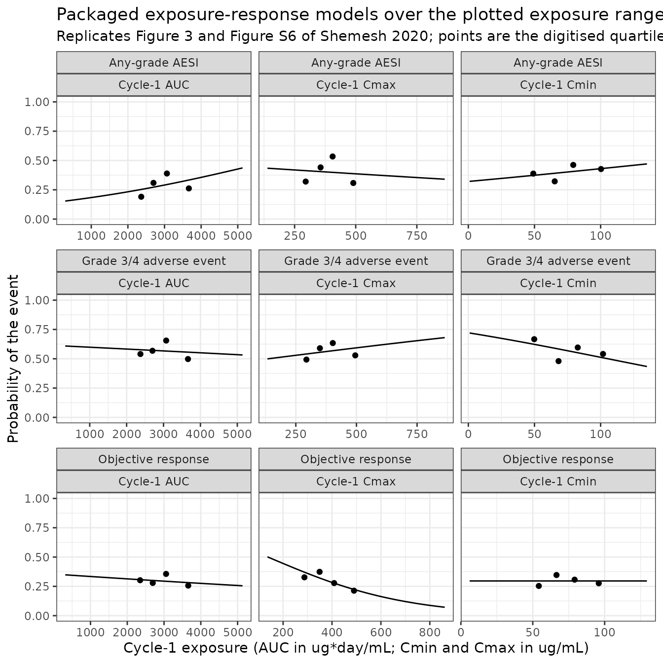

Predicted event probabilities in the simulated cohort

The simulated Cycle-1 exposures from the PKNCA section are passed through each model. The resulting cohort-level probabilities are close to the observed incidences. Figure 3D is the exception, for the reason above.

cohortProb <- lapply(models$Model, function(m) {
  p <- modelParts(m)
  x <- switch(p$cov, AUC_ATEZO = exposure$auclast, CTROUGH = exposure$ctrough,
              CMAX = exposure$cmax)
  data.frame(Model = m, meanProbability = mean(predictAt(m, x)))
}) |>
  bind_rows() |>
  left_join(models, by = "Model")
#> Warning: No omega parameters in the model
#> No omega parameters in the model
#> No omega parameters in the model
#> No omega parameters in the model
#> No omega parameters in the model
#> No omega parameters in the model
#> No omega parameters in the model
#> No omega parameters in the model
#> No omega parameters in the model
knitr::kable(cohortProb[, c("Model", "Endpoint", "Exposure", "meanProbability")], digits = 3,
             caption = "Mean predicted probability in the virtual tTMB-high cohort.")

Mean predicted probability in the virtual tTMB-high cohort.
Model	Endpoint	Exposure	meanProbability
Shemesh_2020_atezolizumab_orr_auc	Objective response	Cycle-1 AUC	0.294
Shemesh_2020_atezolizumab_orr_ctrough	Objective response	Cycle-1 Cmin	0.296
Shemesh_2020_atezolizumab_orr_cmax	Objective response	Cycle-1 Cmax	0.294
Shemesh_2020_atezolizumab_aeg34_auc	Grade 3/4 adverse event	Cycle-1 AUC	0.567
Shemesh_2020_atezolizumab_aeg34_ctrough	Grade 3/4 adverse event	Cycle-1 Cmin	0.551
Shemesh_2020_atezolizumab_aeg34_cmax	Grade 3/4 adverse event	Cycle-1 Cmax	0.566
Shemesh_2020_atezolizumab_aesi_auc	Any-grade AESI	Cycle-1 AUC	0.293
Shemesh_2020_atezolizumab_aesi_ctrough	Any-grade AESI	Cycle-1 Cmin	0.411
Shemesh_2020_atezolizumab_aesi_cmax	Any-grade AESI	Cycle-1 Cmax	0.401

Assumptions and deviations

No printed coefficients. Shemesh 2020 reports only exploratory P values and the fitted curves. All eighteen coefficients were recovered from the figures, as described in “Source trace”. Figure 3 is vector graphics, so its four models are exact to the drawing’s precision. The Figure S6 raster traces have a residual of about one pixel. As an independent check, the maintainers digitised the individual outcomes plotted in Figure 3 (about 90% of the circles are separable) and refitted each logistic regression. The refits gave slopes within about 15% of the curve-derived values and reproduced the printed P values: 0.707 vs .751 (3A), 0.888 vs .998 (3B), 0.787 vs .812 (3C) and 0.257 vs .280 (3D).
Flat ORR-C_min curve. Figure 3B is drawn exactly horizontal, so its slope is encoded as 0. A P value of .998 implies a true estimate below the drawing’s resolution.
Linear, uncentred exposure. The logit is linear in the untransformed exposure; the curvature of the drawn curves supports this and rules out the log-exposure form. The rescaling (per 1000 ug*day/mL for AUC, per 100 ug/mL for C_max, per 10 ug/mL for C_min) is only a presentation choice, matching the sibling Chan_2025_atezolizumab_* models. The intercepts are the logit at zero exposure, outside the observed range.
Figure 3D incidence inconsistency. Documented and asserted above. The curve is transcribed as drawn.
Placeholder residual. Each model declares addSd_<output> <- fixed(0.001) only so that rxode2 accepts an observation statement. The source likelihood is Bernoulli, with no residual and no IIV.
PK layer not re-packaged. Shemesh 2020 re-estimates no PK parameter, and every printed PK term is identical to the fixed intravenous layer of Chan_2025_atezolizumab, which supplies Q, the IIV block and the residual error for the exposure simulation. The primary PK source is Stroh et al.
Virtual cohort. The covariate shapes are assumed (see “Virtual cohort”). All patients receive 1200 mg; the few PCD4989g patients dosed by weight are not represented.
tTMB-response curves (Figure S7) not packaged. Figure S7 plots response, grade 3/4 AE and AESI probability against tTMB. The caption calls the line a “mean model-fitted curve for each TMB record”. Its shape (flat, then a steep rise on a log-tTMB axis for response; flat, then a fall for grade 3/4 AEs) cannot be reproduced by a two-parameter logistic in tTMB, log(tTMB), log(1 + tTMB) or the square root of tTMB (best logit RMSE 0.25, against 0.02 or less for every exposure panel). The x-axis is labelled only at the three quartile boundaries. The underlying model and predictor transform are not stated, so the curves cannot be turned into a model without inventing structure.