Valemetostat concentration-QTc (Tachibana 2025)
Source:vignettes/articles/Tachibana_2025_valemetostat_QTc.Rmd
Tachibana_2025_valemetostat_QTc.RmdModel and source
- Citation: Tachibana M, Poland B, Kakurai Y, Chen Y, Li C, Lau Y. Concentration-QTc Analysis of Valemetostat in Patients With Hematologic Malignancies. Clin Transl Sci. 2025;18(11):e70391. doi:10.1111/cts.70391.
- Article: https://doi.org/10.1111/cts.70391
Tachibana et al. (2025) assessed the QT liability of valemetostat, an oral dual inhibitor of enhancer of zeste homolog 1 and 2 (EZH1/EZH2), from time-matched plasma concentrations and triplicate 12-lead ECGs collected in two phase 1 studies: DS3201-A-J101 (relapsed/refractory B- or T-cell non-Hodgkin lymphoma, 150-300 mg once daily) and DS3201-A-U102 (relapsed/refractory acute myeloid or acute lymphoblastic leukemia, 100-700 mg once daily). A prespecified linear mixed-effects model related the concentration to the change from baseline in the Fridericia-corrected QT interval (DeltaQTcF) and, because Fridericia did not fully remove the heart-rate dependence, in a population-specific corrected QT interval (DeltaQTcP, QTcP = QT / RR^0.443). The package carries one file for each final model:
| Model file | Endpoint | Output | Source table |
|---|---|---|---|
Tachibana_2025_valemetostat_QTcF |
DeltaQTcF (ms) | QTcF |
Table 2 |
Tachibana_2025_valemetostat_QTcP |
DeltaQTcP (ms) | QTcP |
Table 2 |
Both share one structure (Methods, “Data Analysis”):
with correlated additive random effects on the intercept and slope,
and an additive residual error whose SD in U102 is the J101 SD times an
estimated multiplier. There is no placebo arm and no nominal-time
effect, so the typical (mean-covariate) prediction is simply
intercept + slope * concentration, which is how the paper’s
Table 3 was generated.
Covariates in the model files:
-
CP_VALEMETOSTAT_NGML– time-matched valemetostat plasma concentration (ng/mL); 0 at baseline and below the quantification limit. -
QTC_BL– the patient’s pre-dose Cycle 1 Day 1 QTcF (QTcF model) or QTcP (QTcP model), ms. -
STUDY_U102– 1 for U102, 0 for J101; selects the residual SD only.
Both are PD-only models: concentrations enter as data. The registry’s
valemetostat population PK model, Inoue_2025_valemetostat,
predicts total concentration in nmol/L; it would need the valemetostat
molar mass to drive these models, which neither paper states, so this
vignette does not couple them.
Population
The primary analysis set was 100 patients (72 from J101, 28 from U102) with 769 triplicate-averaged ECGs matched to a PK sample taken within 15 min after the ECG (Tachibana 2025 Results and Table 1). Overall, 50% were male; 49% Asian, 41% White, 8% Black and 2% other; mean age 63.8 years (SD 13.4). Mean baseline heart rate was 77.2 bpm (SD 15.4) and mean baseline QTcF 417 ms (SD 24.4). Most patients (56%) received 200 mg once daily. Age, sex, race, study population (NHL versus leukemia) and baseline calcium, potassium and magnesium were screened and none was retained on a fixed effect; only the residual SD differs between the studies.
Source trace
| Element | QTcF model | QTcP model | Source |
|---|---|---|---|
| Model structure | linear mixed-effects equation | same | Methods, “Data Analysis” |
e0 (intercept) |
1.05 ms | -0.00395 ms | Table 2 |
slope |
0.000746 ms/(ng/mL) | 0.000938 ms/(ng/mL) | Table 2 |
e_qtc_bl_e0 (baseline effect) |
-0.266 ms/ms | -0.287 ms/ms | Table 2 |
| IIV SD, intercept | 5.52 ms | 5.35 ms | Table 2 |
| IIV SD, slope | 0.00170 ms/(ng/mL) (printed 0.00710; see Assumptions) | 0.00192 ms/(ng/mL) | Table 2 |
| IIV correlation | 0.0616 | 0.451 | Table 2 |
addSd (J101) |
9.99 ms | 9.94 ms | Table 2 |
e_study_u102_addSd |
1.21 | 1.20 | Table 2 |
| Baseline centering | 417 ms (published mean) | 429 ms (derived) | Table 1; Assumptions |
| QTcP exponent | – | 0.443 | Results, “QT Correction” |
| Validation targets | DeltaQTcF at 9 study/dose Cmax values | DeltaQTcP at the same | Table 3 |
Models
mod_qtcf <- readModelDb("Tachibana_2025_valemetostat_QTcF")
mod_qtcp <- readModelDb("Tachibana_2025_valemetostat_QTcP")
# Only the random effects are zeroed: the residual SD is computed in model()
# (addSd_i, study-specific), so there is no sigma parameter to zero, and the
# typical-value columns used below are predictions without residual error.
mod_qtcf_typ <- rxode2::zeroRe(mod_qtcf, which = "omega")
mod_qtcp_typ <- rxode2::zeroRe(mod_qtcp, which = "omega")

qtcf_ref <- 417
qtcp_ref <- 429

# PD-only event table: no dosing records and no ODE states; every covariate is
# a column. The models are algebraic, so typical-value rows can share one id.
pd_events <- function(conc, qtc_bl, study_u102 = 0) {
  n <- max(length(conc), length(qtc_bl), length(study_u102))
  data.frame(
    id = 1L, time = seq_len(n), evid = 0L, amt = 0,
    CP_VALEMETOSTAT_NGML = rep_len(conc, n),
    QTC_BL = rep_len(qtc_bl, n),
    STUDY_U102 = rep_len(study_u102, n)
  )
}

solve_typ <- function(model, ev) {
  as.data.frame(rxode2::rxSolve(model, events = ev, omega = NA))
}
Structural checks
At the cohort-mean baseline, the typical prediction must equal
e0 + slope * C for any concentration, must move by
e_qtc_bl_e0 per ms of baseline deviation, and must not
depend on the study indicator (which acts on the residual SD only).
These are identities of the encoding and are asserted at machine
precision.
conc_chk <- c(0, 500, 2000, 6000)
bl_chk <- c(-30, 0, 30)
grid <- expand.grid(conc = conc_chk, dbl = bl_chk, study = c(0, 1))

f_qtcf <- solve_typ(mod_qtcf_typ, pd_events(grid$conc, qtcf_ref + grid$dbl, grid$study))$QTcF
f_qtcp <- solve_typ(mod_qtcp_typ, pd_events(grid$conc, qtcp_ref + grid$dbl, grid$study))$QTcP

stopifnot(
  isTRUE(all.equal(f_qtcf, 1.05 + 0.000746 * grid$conc - 0.266 * grid$dbl, tolerance = 1e-12)),
  isTRUE(all.equal(f_qtcp, -0.00395 + 0.000938 * grid$conc - 0.287 * grid$dbl, tolerance = 1e-12))
)
Predicted DeltaQTc at steady-state Cmax (Table 3)
Tachibana 2025 Table 3 gives the model-predicted mean DeltaQTcF and DeltaQTcP at the steady-state geometric mean Cmax of every study and dose, with covariates at their means. The typical models reproduce them.
tab3 <- data.frame(
  study = c(rep("J101", 4), rep("U102", 5)),
  dose = c(150, 200, 250, 300, 100, 150, 250, 500, 700),
  n = c(7, 57, 7, 2, 4, 4, 3, 9, 6),
  cmax = c(1460, 1830, 1510, 3690, 790, 330, 3560, 3970, 4850),
  qtcf_pub = c(2.14, 2.41, 2.18, 3.80, 1.64, 1.30, 3.71, 4.01, 4.67),
  qtcp_pub = c(1.37, 1.71, 1.41, 3.46, 0.74, 0.31, 3.33, 3.72, 4.54)
)
tab3$qtcf_sim <- solve_typ(mod_qtcf_typ, pd_events(tab3$cmax, qtcf_ref))$QTcF
tab3$qtcp_sim <- solve_typ(mod_qtcp_typ, pd_events(tab3$cmax, qtcp_ref))$QTcP

# Table 3 is printed to 0.01 ms; the model reproduces every row to within
# that rounding.
stopifnot(
  max(abs(tab3$qtcf_sim - tab3$qtcf_pub)) < 0.01,
  max(abs(tab3$qtcp_sim - tab3$qtcp_pub)) < 0.01
)

tab3 |>
  dplyr::select(study, dose, n, cmax, qtcf_pub, qtcf_sim, qtcp_pub, qtcp_sim) |>
  dplyr::rename(
    "Study" = study,
    "Dose (mg QD)" = dose,
    "N" = n,
    "Steady-state Cmax (ng/mL)" = cmax,
    "DeltaQTcF published (ms)" = qtcf_pub,
    "DeltaQTcF model (ms)" = qtcf_sim,
    "DeltaQTcP published (ms)" = qtcp_pub,
    "DeltaQTcP model (ms)" = qtcp_sim
  ) |>
knitr::kable(digits = 2, caption = "Replicates Table 3 of Tachibana 2025 (mean predictions).")| Study | Dose (mg QD) | N | Steady-state Cmax (ng/mL) | DeltaQTcF published (ms) | DeltaQTcF model (ms) | DeltaQTcP published (ms) | DeltaQTcP model (ms) |
|---|---|---|---|---|---|---|---|
| J101 | 150 | 7 | 1460 | 2.14 | 2.14 | 1.37 | 1.37 |
| J101 | 200 | 57 | 1830 | 2.41 | 2.42 | 1.71 | 1.71 |
| J101 | 250 | 7 | 1510 | 2.18 | 2.18 | 1.41 | 1.41 |
| J101 | 300 | 2 | 3690 | 3.80 | 3.80 | 3.46 | 3.46 |
| U102 | 100 | 4 | 790 | 1.64 | 1.64 | 0.74 | 0.74 |
| U102 | 150 | 4 | 330 | 1.30 | 1.30 | 0.31 | 0.31 |
| U102 | 250 | 3 | 3560 | 3.71 | 3.71 | 3.33 | 3.34 |
| U102 | 500 | 9 | 3970 | 4.01 | 4.01 | 3.72 | 3.72 |
| U102 | 700 | 6 | 4850 | 4.67 | 4.67 | 4.54 | 4.55 |
Every row agrees to within 0.006 ms, the rounding of the printed values. The 90% confidence intervals of Table 3, and the concentrations at which their upper bound reaches 10 ms (6058 ng/mL for QTcF and 5783 ng/mL for QTcP, Discussion), depend on the sampling covariance of the intercept and slope, which is not reported, so they cannot be reproduced.
conc_grid <- seq(0, 8500, by = 50)
curve_df <- dplyr::bind_rows(
  data.frame(endpoint = "DeltaQTcF (ms)", conc = conc_grid,
             value = solve_typ(mod_qtcf_typ, pd_events(conc_grid, qtcf_ref))$QTcF),
  data.frame(endpoint = "DeltaQTcP (ms)", conc = conc_grid,
             value = solve_typ(mod_qtcp_typ, pd_events(conc_grid, qtcp_ref))$QTcP)
)
pts_df <- dplyr::bind_rows(
  data.frame(endpoint = "DeltaQTcF (ms)", conc = tab3$cmax, value = tab3$qtcf_pub, study = tab3$study),
  data.frame(endpoint = "DeltaQTcP (ms)", conc = tab3$cmax, value = tab3$qtcp_pub, study = tab3$study)
)
ggplot(curve_df, aes(conc, value)) +
  geom_line(colour = "steelblue") +
  geom_point(data = pts_df, aes(colour = study), size = 2) +
  geom_hline(yintercept = 10, linetype = "dotted") +
  facet_wrap(~endpoint) +
  labs(x = "Valemetostat concentration (ng/mL)", y = "Change from baseline (ms)", colour = "Study") +
  theme_bw()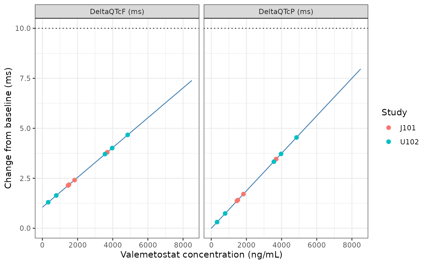
Typical DeltaQTc across the observed concentration range. Replicates the mean lines of Figure 2 of Tachibana 2025; points are the Table 3 predictions at the steady-state Cmax values, and the dotted line is the 10 ms threshold.
Virtual cohort and stochastic simulation
To exercise the random effects and the study-specific residual error, a virtual cohort of 200 patients per study is simulated with seven post-baseline ECGs each (Cycle 1 Day 1 at 1, 2 and 8 h; Cycle 1 Day 8/15 pre-dose and at 1, 2 and 8 h). Each record’s concentration is drawn from a log-normal distribution whose mean and SD match the pooled observed concentrations at that timepoint (Tachibana 2025 Table S1). Baseline QTcF and heart rate are drawn per study from normal distributions with the Table 1 means and SDs, and each patient’s baseline QTcP is computed from them with the 0.443 exponent (QTcP = QTcF * RR^(1/3 - 0.443)).
set.seed(20251118)
n_per_study <- 200

# Table S1 pooled concentration mean / SD (ng/mL) by timepoint
tp <- data.frame(
  timepoint = c("C1D1 H1", "C1D1 H2", "C1D1 H8", "C1D8/15 H0", "C1D8/15 H1", "C1D8/15 H2", "C1D8/15 H8"),
  mean = c(1122, 1665, 956, 519, 1349, 1910, 1323),
  sd = c(1279, 1722, 880, 782, 1165, 1755, 1602)
)
tp$sdlog <- sqrt(log(1 + (tp$sd / tp$mean)^2))
tp$meanlog <- log(tp$mean) - tp$sdlog^2 / 2

# Table 1 baseline means / SDs by study
bl_par <- data.frame(
  STUDY_U102 = c(0, 1),
  qtcf_mean = c(417, 416), qtcf_sd = c(26.9, 17.0),
  hr_mean = c(74.9, 83.3), hr_sd = c(15.5, 13.7)
)
patients <- data.frame(
  id = seq_len(2 * n_per_study),
  STUDY_U102 = rep(c(0, 1), each = n_per_study)
) |>
  dplyr::left_join(bl_par, by = "STUDY_U102") |>
  dplyr::mutate(
    qtcf_bl = rnorm(dplyr::n(), qtcf_mean, qtcf_sd),
    hr_bl = pmin(pmax(rnorm(dplyr::n(), hr_mean, hr_sd), 45), 130),
    qtcp_bl = qtcf_bl * (60 / hr_bl)^(1 / 3 - 0.443)
  ) |>
  dplyr::select(id, STUDY_U102, qtcf_bl, qtcp_bl)

cohort <- merge(patients, data.frame(tp_index = seq_len(nrow(tp))), by = NULL) |>
  dplyr::arrange(id, tp_index) |>
  dplyr::mutate(
    time = tp_index,
    CP_VALEMETOSTAT_NGML = rlnorm(dplyr::n(), tp$meanlog[tp_index], tp$sdlog[tp_index]),
    evid = 0L, amt = 0
  )

ev_qtcf <- cohort |>
  dplyr::transmute(id, time, evid, amt, CP_VALEMETOSTAT_NGML, QTC_BL = qtcf_bl, STUDY_U102)
ev_qtcp <- cohort |>
  dplyr::transmute(id, time, evid, amt, CP_VALEMETOSTAT_NGML, QTC_BL = qtcp_bl, STUDY_U102)

sim_qtcf <- as.data.frame(rxode2::rxSolve(mod_qtcf, events = ev_qtcf))
sim_qtcp <- as.data.frame(rxode2::rxSolve(mod_qtcp, events = ev_qtcp))

summary(cohort$qtcp_bl)
#>    Min. 1st Qu.  Median    Mean 3rd Qu.    Max.
#>   337.3   414.2   428.3   428.5   445.9   491.2
The simulated mean baseline QTcP is close to the 429 ms centering value used by the QTcP model (see Assumptions).
sim_long <- dplyr::bind_rows(
  sim_qtcf |> dplyr::transmute(id, conc = CP_VALEMETOSTAT_NGML, QTC_BL, STUDY_U102,
                               endpoint = "DeltaQTcF (ms)", sim, ref = qtcf_ref),
  sim_qtcp |> dplyr::transmute(id, conc = CP_VALEMETOSTAT_NGML, QTC_BL, STUDY_U102,
                               endpoint = "DeltaQTcP (ms)", sim, ref = qtcp_ref)
) |>
  dplyr::mutate(study = ifelse(STUDY_U102 == 1, "U102", "J101"))

ggplot(sim_long, aes(conc, sim, colour = study)) +
  geom_point(alpha = 0.25, size = 0.8) +
  geom_line(data = curve_df, aes(conc, value), colour = "black", inherit.aes = FALSE) +
  geom_hline(yintercept = 10, linetype = "dotted") +
  facet_wrap(~endpoint) +
  scale_colour_manual(values = c(J101 = "steelblue", U102 = "seagreen")) +
  coord_cartesian(xlim = c(0, 8500)) +
  labs(x = "Valemetostat concentration (ng/mL)", y = "Simulated change from baseline (ms)", colour = "Study") +
  theme_bw()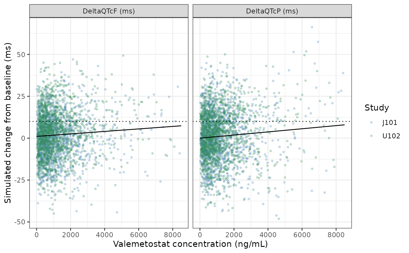
Simulated DeltaQTc against concentration with the typical-value line. Replicates the layout of Figure 1B / Figure 2 of Tachibana 2025 (J101 blue, U102 green).
Checks on the stochastic simulation
Two properties are checked. First, the random effects and residual error have zero mean, so the simulated values must scatter around the typical prediction evaluated at each record’s own concentration and baseline. Second, the residual SD (simulated value minus individual prediction) must be about 9.99 ms (QTcF) or 9.94 ms (QTcP) in J101 and 1.21 or 1.20 times that in U102. With 1400 records per study the standard error of an SD estimate is about 2%, so a 10% tolerance is wide against sampling noise and narrow against a dropped or inverted study multiplier (a 20% shift).
typ_qtcf <- solve_typ(mod_qtcf_typ, ev_qtcf |> dplyr::mutate(id = 1L, time = seq_len(dplyr::n())))$QTcF
typ_qtcp <- solve_typ(mod_qtcp_typ, ev_qtcp |> dplyr::mutate(id = 1L, time = seq_len(dplyr::n())))$QTcP

resid_sd <- dplyr::bind_rows(
  sim_qtcf |> dplyr::transmute(endpoint = "QTcF", STUDY_U102, res = sim - QTcF),
  sim_qtcp |> dplyr::transmute(endpoint = "QTcP", STUDY_U102, res = sim - QTcP)
) |>
  dplyr::group_by(endpoint, STUDY_U102) |>
  dplyr::summarise(sd_sim = stats::sd(res), .groups = "drop") |>
  dplyr::mutate(
    sd_model = dplyr::case_when(
      endpoint == "QTcF" & STUDY_U102 == 0 ~ 9.99,
      endpoint == "QTcF" & STUDY_U102 == 1 ~ 9.99 * 1.21,
      endpoint == "QTcP" & STUDY_U102 == 0 ~ 9.94,
      TRUE ~ 9.94 * 1.20
    ),
    pct_diff = 100 * (sd_sim - sd_model) / sd_model
  )

mean_dev <- c(
  QTcF = mean(sim_qtcf$sim - typ_qtcf),
  QTcP = mean(sim_qtcp$sim - typ_qtcp)
)

stopifnot(
  all(abs(resid_sd$pct_diff) < 10),
  # Standard error of the mean deviation is about 0.3 ms (intercept SD ~5.5 ms
  # over 400 patients, residual SD ~11 ms over 2800 records).
  all(abs(mean_dev) < 1.5)
)

resid_sd |>
  dplyr::mutate(study = ifelse(STUDY_U102 == 1, "U102", "J101")) |>
  dplyr::select(endpoint, study, sd_model, sd_sim, pct_diff) |>
  dplyr::rename(
    "Endpoint" = endpoint,
    "Study" = study,
    "Model residual SD (ms)" = sd_model,
    "Simulated residual SD (ms)" = sd_sim,
    "% diff" = pct_diff
  ) |>
knitr::kable(digits = 2, caption = "Residual SD by study in the simulated cohort.")| Endpoint | Study | Model residual SD (ms) | Simulated residual SD (ms) | % diff |
|---|---|---|---|---|
| QTcF | J101 | 9.99 | 9.77 | -2.21 |
| QTcF | U102 | 12.09 | 12.03 | -0.52 |
| QTcP | J101 | 9.94 | 9.75 | -1.86 |
| QTcP | U102 | 11.93 | 12.13 | 1.70 |
knitr::kable(
  data.frame(Endpoint = names(mean_dev), "Mean simulated minus typical (ms)" = unname(mean_dev),
             check.names = FALSE),
  digits = 2
)| Endpoint | Mean simulated minus typical (ms) |
|---|---|
| QTcF | -0.12 |
| QTcP | 0.18 |
NCA
The models take concentration as an input and contain no dosing or PK, so there is no concentration-time profile to analyse and PKNCA does not apply. The exposure values the paper uses (the steady-state Cmax of Table 3) come from the valemetostat PK analyses of the two studies, and are used directly as model inputs above.
Assumptions and deviations
- Slope random-effect SD (QTcF). Table 2 prints the SD of the slope random effect as 0.00710 ms/(ng/mL). Its standard error (0.000518) and relative standard error (30.5%) give 0.000518 / 0.305 = 0.00170, and its 95% CI (0.000865 to 0.00266) is centered near 0.0017 and excludes 0.00710. The QTcP model (0.00192) and the sensitivity model of Table S2 (0.00201) are also of that size. The model uses 0.00170, treating 0.00710 as a transposition of digits.
-
QTcP centering constant. The models centre baseline
QTc on the mean over all patients. For QTcF this is published (417 ms,
Table 1). For QTcP it is not, so 429 ms is derived from the Table 1
means as 417 * (60 / 77.2)^(1/3 - 0.443) = 428.7 ms. The simulated
cohort above, which computes QTcP per patient, has a mean within about 1
ms of this value. An error of 1 ms in the constant shifts a prediction
by 0.29 ms; it does not affect the typical prediction at
QTC_BL = 429. - Correlation estimates. Table 2 gives the intercept-slope correlations (0.0616 for QTcF, 0.451 for QTcP) without standard errors; they are used as printed.
- Abstract versus Results on slope significance. The abstract states that the slope was significant for DeltaQTcF but not DeltaQTcP; Table 2 and the Results state the reverse (the DeltaQTcF 95% CI includes 0, the DeltaQTcP CI excludes it). The model files follow Table 2; neither statement changes a parameter value.
- Patient counts. Table 3 lists 57 patients at 200 mg in J101 and 9 and 6 at 500 and 700 mg in U102, whereas Table 1 lists 56, 10 and 7. The counts are reproduced from Table 3 for display only and do not enter any calculation.
- Not packaged. The base model and the timepoint-match sensitivity model (Table S2, 1166 ECGs) are not packaged; the paper presents them as supporting analyses of the final models.
- Virtual cohort. The log-normal concentration draws, the truncation of heart rate at 45-130 bpm and the independence of concentration and baseline are assumptions of this vignette; the dose of each simulated patient is not represented.
- Metabolite. Only parent valemetostat concentrations were modelled; the major metabolite CALZ-1809a was not included.