Model and source
mod <- readModelDb("Du_2022_busulfan")
cat(rxode2::rxode(mod)$reference)
#> ℹ parameter labels from comments will be replaced by 'label()'
#> Du X, Huang C, Xue L, Jiao Z, Zhu M, Li J, Lu J, Xiao P, Zhou X, Mao C, Zhu Z, Dong J, Liu X, Chen Z, Zhang S, Ding Y, Hu S, Miao L. The Correlation Between Busulfan Exposure and Clinical Outcomes in Chinese Pediatric Patients: A Population Pharmacokinetic Study. Front Pharmacol. 2022;13:905879. doi:10.3389/fphar.2022.905879- Article: https://doi.org/10.3389/fphar.2022.905879
- Supplementary material (Supplementary Equations S1-S8 and Tables S1-S6): DataSheet1 at the article landing page.
Du 2022 developed a one-compartment population PK model for intravenous busulfan in Chinese children undergoing hematopoietic stem cell transplantation (HSCT), then used the individual exposures it predicted to look for an exposure window associated with event-free survival. Clearance is scaled by an allometric normal fat mass (NFM, exponent fixed at 3/4, with an estimated fat fraction) and by a sigmoid maturation function of postmenstrual age (PMA). Volume is scaled linearly by fat-free mass (FFM). Nine candidate NFM size models were compared (Table 1), and Model III was carried forward as the final model (Table 2).
Population
The model was fitted to 467 plasma concentrations from 128 children who received IV busulfan (Busulfex) at the Children’s Hospital of Soochow University between July 2018 and February 2021 (Methods; Supplementary Table S3). Mean postnatal age was 6.11 years (range 0.6-17.0), mean weight 23.99 kg (7.5-96.5), mean height 115.1 cm (67-185) and mean gestational age 39.8 weeks (32-40). Seventy percent were male and 70% had a malignant disease. Busulfan was dosed at 0.8, 1.0 or 1.2 mg/kg per dose (112, 13 and 3 patients, Supplementary Table S2) as a 2 h infusion four times daily for 2, 3 or 4 days. Samples were drawn 0, 2 and 4 h after the end of the first infusion, with a pre-dose sample before the fifth dose in 61 patients.
The exposure-outcome analysis used the 63 patients on the 16-dose regimen (Table 3): median age 2.5 years (0.6-16.9), median weight 14.4 kg (7-63), 69.8% male, and a median model-predicted busulfan AUC of 1425.4 uM x min (range 691.5-2156.0).
str(mod()$population)
#> List of 16
#>  $ species       : chr "human"
#>  $ n_subjects    : num 128
#>  $ n_studies     : num 1
#>  $ n_centers     : num 1
#>  $ n_observations: num 467
#>  $ age_range     : chr "0.6-17.0 years (mean 6.11)"
#>  $ weight_range  : chr "7.5-96.5 kg (mean 23.99)"
#>  $ height_range  : chr "67-185 cm (mean 115.11)"
#>  $ ga_range      : chr "32-40 weeks (mean 39.82)"
#>  $ pma_range     : chr "70.6-926 weeks (mean 368.32)"
#>  $ sex_female_pct: num 29.7
#>  $ race_ethnicity: chr "Chinese"
#>  $ disease_state : chr "Pediatric patients receiving IV busulfan as part of conditioning before hematopoietic stem cell transplantation"| __truncated__
#>  $ dose_range    : chr "0.8, 1.0 or 1.2 mg/kg per dose (actual or adjusted body weight), 2 h IV infusion four times daily for 2-4 days (8-16 doses)"
#>  $ regions       : chr "China (Children's Hospital of Soochow University, Suzhou)"
#>  $ notes         : chr "Patients enrolled July 2018 to February 2021 (Methods). Sampling at 0, 2 and 4 h after the end of the first 2 h"| __truncated__
Source trace
Every ini() value carries an in-file comment pointing to
its source. The table collects them, together with the equations in
model().
| Element | Value | Source |
|---|---|---|
lcl (CL_STD) |
log(7.71 L/h) | Table 2 (= Table 1 Model III) |
lvc (V_STD) |
log(42.4 L) | Table 2 |
ffat_cl (Ffat_CL) |
0.692 | Table 2 |
e_nfm_cl (k1) |
0.75, fixed | Methods; Table 1 Model III |
tm50_mat (TM50) |
31.0 weeks | Table 2 |
hill_mat (HILL) |
2.03 | Table 2 |
etalcl (BSV_CL) |
0.234^2 | Table 2; Results “23.4%” |
etalvc (BSV_V) |
0.240^2 | Table 2; Results “24.0%” |
propSd (RUV_PROP) |
0.130 | Table 2 |
addSd (RUV_ADD) |
0.048 mg/L | Table 2 |
| CL = CL_STD x (NFM / NFM_STD)^k1 x Fmat | Equation 1 | |
| V = V_STD x (NFM / NFM_STD), Ffat_V = 0 so NFM = FFM | Equation 2; Results | |
| FFM = WHSmax x HT^2 x WT / (WHS50 x HT^2 + WT) | Supplementary Equation S3 | |
| NFM = FFM + Ffat x (WT - FFM) | Supplementary Equation S4 | |
| Fmat = 1 / (1 + (PMA / TM50)^-Hill) | Supplementary Equation S5 | |
| PMA = AGE x 52 + GA | Supplementary Equation S6 | |
| FFM_STD = 56.1 kg (70 kg, 176 cm male) | Table 1 and 2 footnotes | |
| Y = C + sqrt(C^2 x prop^2 + add^2) x eps | Supplementary Equation S2 |
The model takes FFM as a data column. The helper below
implements Supplementary Equation S3, which is how the paper computed it
(height in metres).
ffm_janmahasatian <- function(WT, HT_cm, SEXF) {
  ht2 <- (HT_cm / 100)^2
  ifelse(
    SEXF == 1,
    37.99 * ht2 * WT / (35.98 * ht2 + WT),
    42.92 * ht2 * WT / (30.93 * ht2 + WT)
  )
}
# The standard subject: a 70 kg, 176 cm male has FFM 56.1 kg.
ffm_std <- ffm_janmahasatian(70, 176, 0)
ffm_std
#> [1] 56.12749
stopifnot(abs(ffm_std - 56.1) < 0.05)
Closed-form checks
With all random effects at zero, the standard adult (70 kg, 176 cm, male, 30 years old, born at 40 weeks, FFM set to the paper’s FFM_STD of 56.1 kg) must return the Table 2 typical values. His NFM equals the standard NFM, and his maturation fraction is essentially 1.
typ <- rxode2::zeroRe(mod)
#> ℹ parameter labels from comments will be replaced by 'label()'
std_adult <- data.frame(
  id = 1, time = c(0, 1), evid = c(1, 0), amt = c(1, 0), cmt = "central",
  WT = 70, FFM = 56.1, AGE = 30, GA = 40
)
s_std <- rxode2::rxSolve(typ, std_adult, returnType = "data.frame")
#> ℹ omega/sigma items treated as zero: 'etalcl', 'etalvc'
s_std <- s_std[nrow(s_std), ]
c(cl = s_std$cl, vc = s_std$vc, fmat = s_std$fmat)
#>         cl         vc       fmat
#>  7.7074295 42.4000000  0.9996666
stopifnot(
  abs(s_std$cl - 7.71 * s_std$fmat) < 1e-6,
  abs(s_std$fmat - 1) < 1e-3,
  abs(s_std$vc - 42.4) < 1e-6
)
The maturation function reaches half of the adult clearance at a postmenstrual age of 31 weeks, so by the youngest patient in the cohort (0.6 years, about 71 weeks PMA) it already exceeds 80%.
pma <- seq(20, 400, by = 1)
fmat <- 1 / (1 + (pma / 31)^(-2.03))
ggplot(data.frame(pma, fmat), aes(pma, fmat)) +
  geom_line() +
  geom_vline(xintercept = c(70.6), linetype = "dashed") +
  labs(x = "Postmenstrual age (weeks)", y = "Fraction of adult CL")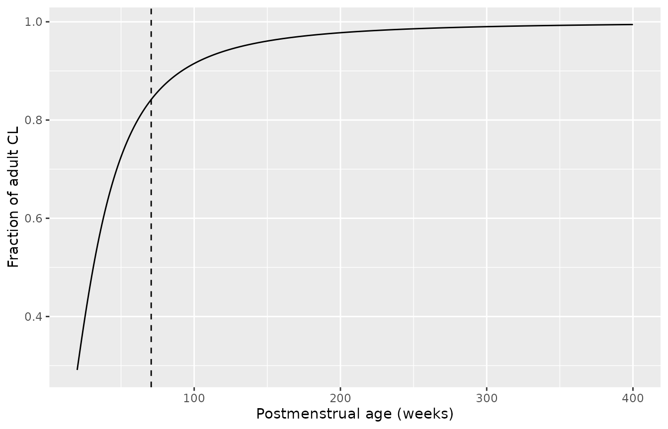
Maturation fraction of busulfan clearance against postmenstrual age (Supplementary Equation S5, TM50 = 31 weeks, Hill = 2.03). The dashed line marks the youngest PMA in the cohort, 70.6 weeks (Supplementary Table S3).
Check against the patients in Supplementary Table S6
Supplementary Table S6 lists sex, age, weight and the model-predicted busulfan AUC of the 16 patients who had an event. Height and dose are not listed. Assuming the predominant 0.8 mg/kg dose (112 of 128 patients) and an approximate median height for age, the typical-value AUC (Dose / CL, which equals the steady-state AUC over one dosing interval) can be computed for each patient. The paper’s values are individual (post hoc) predictions, so they scatter around the typical value with the 23.4% between-subject variability of CL. Their geometric mean ratio to the typical value should therefore sit near 1.
mw_busulfan <- 246.3 # g/mol
to_umol_min <- 1000 / mw_busulfan * 60 # mg*h/L -> uM*min

s6 <- data.frame(
  SEXF = c(0, 0, 1, 0, 0, 1, 0, 0, 0, 1, 0, 0, 1, 0, 0, 0),
  AGE = c(3.8, 2.0, 0.8, 0.9, 1.4, 11.7, 2.2, 7.2, 11.3, 3.6, 10.6, 11.6, 5.1, 1.9, 16.9, 2.3),
  WT = c(16, 11, 8, 8.8, 10, 43, 12, 19.6, 44, 11.5, 32.5, 29, 17, 14.8, 63, 13.5),
  auc_paper = c(
    691.47, 722.36, 751.01, 851.33, 1173.59, 1384.85, 1427.04, 1455.66,
    1497.73, 1514.93, 1518.61, 1632.72, 1643.05, 1797.93, 1877.61, 2155.96
  )
)

# Approximate median height-for-age (cm). The paper does not list heights.
height_for_age <- function(age) {
  approx(
    x = c(0.5, 1, 2, 3, 4, 5, 6, 8, 10, 12, 14, 16, 17),
    y = c(67, 76, 87, 96, 103, 110, 116, 128, 138, 149, 163, 173, 176),
    xout = age, rule = 2
  )$y
}

s6_ev <- s6 |>
  mutate(
    id = row_number(),
    HT = height_for_age(AGE),
    FFM = ffm_janmahasatian(WT, HT, SEXF),
    GA = 40,
    dose = 0.8 * WT
  )
s6_ev <- bind_rows(
  s6_ev |> mutate(time = 0, evid = 1, amt = dose),
  s6_ev |> mutate(time = 1, evid = 0, amt = 0)
) |>
  mutate(cmt = "central") |>
  arrange(id, time)

s6_sim <- rxode2::rxSolve(typ, s6_ev, returnType = "data.frame") |>
  filter(time == 1) |>
  select(id, cl)
#> ℹ omega/sigma items treated as zero: 'etalcl', 'etalvc'
#> Warning: multi-subject simulation without without 'omega'

s6_cmp <- s6 |>
  mutate(id = row_number()) |>
  left_join(s6_sim, by = "id") |>
  mutate(
    auc_typical = 0.8 * WT / cl * to_umol_min,
    ratio = auc_paper / auc_typical
  )

s6_cmp |>
  transmute(
    Sex = ifelse(SEXF == 1, "F", "M"), AGE, WT,
    `Paper AUC (uM x min)` = round(auc_paper),
    `Typical AUC, 0.8 mg/kg (uM x min)` = round(auc_typical),
    `Ratio` = round(ratio, 2)
  ) |>
knitr::kable(caption = "Supplementary Table S6 patients: paper (post hoc) AUC against the typical-value AUC from this model.")| Sex | AGE | WT | Paper AUC (uM x min) | Typical AUC, 0.8 mg/kg (uM x min) | Ratio |
|---|---|---|---|---|---|
| M | 3.8 | 16.0 | 691 | 1207 | 0.57 |
| M | 2.0 | 11.0 | 722 | 1124 | 0.64 |
| F | 0.8 | 8.0 | 751 | 1191 | 0.63 |
| M | 0.9 | 8.8 | 851 | 1152 | 0.74 |
| M | 1.4 | 10.0 | 1174 | 1133 | 1.04 |
| F | 11.7 | 43.0 | 1385 | 1618 | 0.86 |
| M | 2.2 | 12.0 | 1427 | 1146 | 1.25 |
| M | 7.2 | 19.6 | 1456 | 1240 | 1.17 |
| M | 11.3 | 44.0 | 1498 | 1569 | 0.95 |
| F | 3.6 | 11.5 | 1515 | 1146 | 1.32 |
| M | 10.6 | 32.5 | 1519 | 1427 | 1.06 |
| M | 11.6 | 29.0 | 1633 | 1367 | 1.19 |
| F | 5.1 | 17.0 | 1643 | 1266 | 1.30 |
| M | 1.9 | 14.8 | 1798 | 1245 | 1.44 |
| M | 16.9 | 63.0 | 1878 | 1711 | 1.10 |
| M | 2.3 | 13.5 | 2156 | 1186 | 1.82 |
gm_ratio <- exp(mean(log(s6_cmp$ratio)))
gm_ratio
#> [1] 1.018206
# Structural check: a mis-specified size or maturation term, or a misread
# reference NFM, moves this geometric mean by 10-15% or more.
stopifnot(gm_ratio > 0.9, gm_ratio < 1.1)
The geometric mean ratio is close to 1. The spread of the individual ratios is wider than the 23.4% BSV because these 16 patients were selected by having an event, and the exposure-outcome analysis found events concentrated at both ends of the AUC range.
Virtual cohort
A virtual cohort resembling the 63 patients on the 16-dose regimen (Table 3) is built from an age distribution centred on 2.5 years and truncated to 0.6-16.9 years. Height comes from the same approximate height-for-age curve, and weight from a body-mass index of about 16 kg/m^2 with 10% variability. 70% of subjects are male and all were born at 40 weeks.
set.seed(2022)
rxode2::rxSetSeed(2022)
n_sub <- 200
cohort <- tibble(
  id = seq_len(n_sub),
  AGE = pmin(pmax(exp(rnorm(n_sub, log(2.5), 0.85)), 0.6), 16.9),
  SEXF = rbinom(n_sub, 1, 0.3),
  GA = 40
) |>
  mutate(
    HT = height_for_age(AGE) * exp(rnorm(n_sub, 0, 0.04)),
    WT = 16 * (HT / 100)^2 * exp(rnorm(n_sub, 0, 0.1)),
    FFM = ffm_janmahasatian(WT, HT, SEXF),
    dose = 0.8 * WT
  )

cohort |>
  summarise(
    `Median age (y)` = median(AGE),
    `Age range (y)` = paste(round(range(AGE), 1), collapse = "-"),
    `Median weight (kg)` = median(WT),
    `Weight range (kg)` = paste(round(range(WT), 1), collapse = "-"),
    `Male (%)` = 100 * mean(SEXF == 0)
  ) |>
knitr::kable(digits = 1, caption = "Virtual cohort summary (compare Table 3: median 2.5 y and 14.4 kg).")| Median age (y) | Age range (y) | Median weight (kg) | Weight range (kg) | Male (%) |
|---|---|---|---|---|
| 2.6 | 0.6-16.9 | 13.4 | 6.6-58.1 | 69.5 |
Simulation
Each subject receives 0.8 mg/kg as a 2 h infusion every 6 h for 16 doses. Concentrations are recorded densely over the first and the last dosing interval.
dose_times <- seq(0, 90, by = 6)
obs_times <- sort(unique(c(seq(0, 6, by = 0.25), seq(90, 96, by = 0.25), 24)))

doses <- cohort |>
  tidyr::crossing(time = dose_times) |>
  mutate(evid = 1, amt = dose, dur = 2)
obs <- cohort |>
  tidyr::crossing(time = obs_times) |>
  mutate(evid = 0, amt = 0, dur = 0)
ev <- bind_rows(doses, obs) |>
  mutate(cmt = "central") |>
  arrange(id, time, desc(evid)) |>
  as.data.frame()

sim <- rxode2::rxSolve(mod, ev, keep = "dose", returnType = "data.frame")
#> ℹ parameter labels from comments will be replaced by 'label()'
sim |>
  filter(time <= 6) |>
  group_by(time) |>
  summarise(
    p05 = quantile(sim, 0.05), p50 = median(sim), p95 = quantile(sim, 0.95),
    .groups = "drop"
  ) |>
  ggplot(aes(time, p50)) +
  geom_ribbon(aes(ymin = p05, ymax = p95), alpha = 0.25) +
  geom_line() +
  labs(x = "Time after start of first infusion (h)", y = "Busulfan (mg/L)")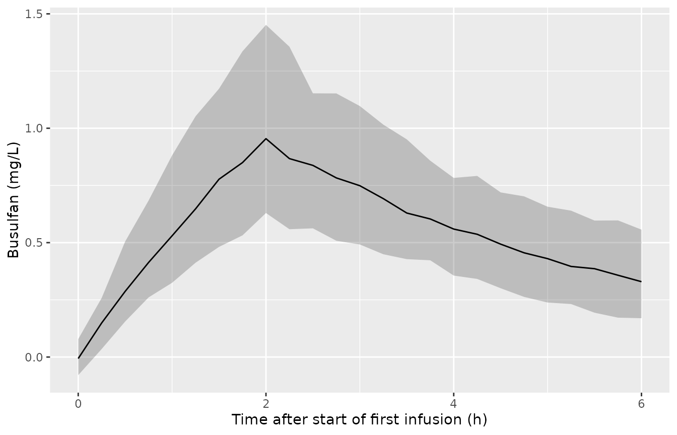
Simulated busulfan concentrations over the first dosing interval (median and 5th-95th percentiles, with residual error). The paper sampled at 2, 4 and 6 h after the start of the first infusion; compare the prediction-corrected VPC in Figure 2 of Du 2022.
PKNCA validation
NCA is run on the individual predictions (Cc, without
residual error) over the first dosing interval and over the 16th dosing
interval at steady state.
conc_df <- sim |>
  filter(!is.na(Cc)) |>
  mutate(treatment = "0.8 mg/kg q6h x16") |>
  select(id, time, Cc, treatment)

dose_df <- doses |>
  filter(time %in% c(0, 90)) |>
  mutate(treatment = "0.8 mg/kg q6h x16") |>
  select(id, time, amt, treatment)

conc_obj <- PKNCA::PKNCAconc(conc_df, Cc ~ time | treatment + id)
dose_obj <- PKNCA::PKNCAdose(dose_df, amt ~ time | treatment + id)
intervals <- data.frame(
  start = c(0, 90), end = c(6, 96),
  cmax = TRUE, auclast = TRUE, cmin = c(FALSE, TRUE)
)
nca_res <- PKNCA::pk.nca(PKNCA::PKNCAdata(conc_obj, dose_obj, intervals = intervals))

nca_tbl <- as.data.frame(nca_res$result) |>
  group_by(start, PPTESTCD) |>
  summarise(median = median(PPORRES), .groups = "drop") |>
  pivot_wider(names_from = PPTESTCD, values_from = median)
nca_tbl |>
  mutate(Interval = ifelse(start == 0, "Dose 1 (0-6 h)", "Dose 16 (90-96 h)")) |>
  select(Interval, cmax, auclast, cmin) |>
  rename(
    "Cmax (mg/L)" = cmax,
    "AUC over the interval (mg*h/L)" = auclast,
    "Cmin (mg/L)" = cmin
  ) |>
knitr::kable(digits = 3, caption = "Median simulated NCA by dosing interval.")| Interval | Cmax (mg/L) | AUC over the interval (mg*h/L) | Cmin (mg/L) |
|---|---|---|---|
| Dose 1 (0-6 h) | 0.954 | 3.385 | NA |
| Dose 16 (90-96 h) | 1.256 | 4.878 | 0.426 |
For a linear model the steady-state AUC over one interval equals Dose / CL, so the dose-16 AUC is the same quantity as the per-dose busulfan AUC the paper reports. Table 3 gives a median of 1425.4 uM x min in the 63-patient 16-dose subgroup.
sim_ss <- as.data.frame(nca_res$result) |>
  filter(start == 90, PPTESTCD == "auclast") |>
  mutate(treatment = "0.8 mg/kg q6h x16")

ref <- data.frame(treatment = "0.8 mg/kg q6h x16", auclast = 1425.4 / to_umol_min)

cmp <- nlmixr2lib::ncaComparisonTable(
  simulated = sim_ss[, c("treatment", "PPTESTCD", "PPORRES")],
  reference = ref,
  by = "treatment",
  units = c(auclast = "mg*h/L"),
  tolerance_pct = 20
)
knitr::kable(cmp, caption = "Median steady-state AUC over one 6 h interval against Table 3 (1425.4 uM x min = 5.85 mg*h/L).")| NCA parameter | treatment | Reference | Simulated | % diff |
|---|---|---|---|---|
| AUClast (mg*h/L) | 0.8 mg/kg q6h x16 | 5.85 | 4.88 | -16.6% |
sim_med_auc <- median(sim_ss$PPORRES) * to_umol_min
sim_med_auc
#> [1] 1188.365
# Robust centre only: the cohort's per-dose mg/kg mix is unknown (see below).
stopifnot(abs(sim_med_auc / 1425.4 - 1) < 0.3)
The simulated median sits below the paper’s 1425.4 uM x min. Two things explain most of the gap, and both concern the cohort rather than the model. First, the paper does not report the per-dose mg/kg mix within the 16-dose subgroup. The 16 patients on 1.0 or 1.2 mg/kg were the lighter ones (mean weight 14.65 and 12.67 kg, Supplementary Table S2), so the young 16-dose subgroup probably holds most of them, and its average dose exceeds the 0.8 mg/kg simulated here. Second, the virtual heights and weights are approximations. The Supplementary Table S6 check above, which uses actual patient ages and weights, agrees much more closely.
Assumptions and deviations
-
Reference NFM for clearance. Equation 1 divides NFM
by NFM_STD, which the Methods say was “calculated using Supplementary
Equations S3, S4” for the 70 kg, 176 cm standard male. With Ffat_CL =
0.692 that is 56.1 + 0.692 x (70 - 56.1) = 65.7 kg, and this is what the
model uses. Table 1 writes the model description in shorthand as “CL x
(NFM/56.1)^3/4”, where 56.1 kg is FFM_STD. Two pieces of evidence favour
the equation:
- the paper reports CL_STD as the clearance of the 70 kg standard adult, which holds only if NFM_STD is computed with Ffat; (ii) in the Supplementary Table S6 check, the equation reading gives a geometric mean ratio near 1. With a fixed 56.1 kg denominator, the ratio rises to about 1.15, because typical clearance at every size is 12.6% higher ((65.7 / 56.1)^0.75).
- BSV scale. Table 2 reports BSV_CL = 0.234 and BSV_V = 0.240, and the Results describe them as 23.4% and 24.0%. They are read as the SD of eta, so omega^2 = 0.0548 and 0.0576. Reading them as CVs (omega^2 = log(CV^2 + 1)) would give 0.0533 and 0.0560, a difference of under 3%.
-
Residual error. Supplementary Equation S2 adds the
proportional and additive variances, which is the nlmixr2 default
combined2form ofadd() + prop(). -
Volume. The fat fraction for V was zero (Results),
so V scales linearly on FFM with FFM_STD = 56.1 kg. No
ffatparameter for V is carried, because Table 2 lists none. - Between-occasion variability. BOV on CL and V was tested and not retained (Supplementary Table S5 rows 20-21), so the model has none.
-
FFM is an input column. The paper derives FFM with
the adult Janmahasatian equation (Supplementary Equation S3) for all
ages and applies no paediatric correction. The vignette helper
ffm_janmahasatian()reproduces it. - PMA uses 52 weeks per year, as written in Supplementary Equation S6.
- Exposure-outcome analysis not encoded. The event-free-survival analysis is a Cox proportional-hazards regression (quadratic in log AUC, and a categorical 950-1,600 uM x min window with HR 0.32). The paper reports neither a baseline hazard nor the quadratic coefficients, so there is no simulable time-to-event model to extract. The toxicity logistic regressions were not significant.
- Virtual cohort. Heights come from an approximate median height-for-age curve and weights from a BMI near 16 kg/m^2, because the paper reports only summary demographics. Gestational age is set to 40 weeks (cohort mean 39.8 weeks). All simulated subjects receive 0.8 mg/kg per dose.
- Errata. No erratum or correction for this article was found (checked 2026-10-02).