Lopinavir (Thoueille 2023)
Source:vignettes/articles/Thoueille_2023_lopinavir.Rmd
Thoueille_2023_lopinavir.RmdModel and source
- Citation: Thoueille P, Delfraysse M, Andre P, Buclin T, Decosterd LA, Fedeli C, Ustero P, Calmy A, Guidi M; Swiss HIV Cohort Study. Population pharmacokinetic analysis of lopinavir in HIV negative individuals exposed to SARS-CoV-2: a COPEP (COronavirus Post-Exposure Prophylaxis) sub-study. BMC Pharmacol Toxicol. 2023;24:47. doi:10.1186/s40360-023-00687-6
- Description: One-compartment first-order-absorption population PK model for oral ritonavir-boosted lopinavir (LPV/r) in HIV-negative individuals receiving 5-day COVID-19 post-exposure prophylaxis (COPEP study) pooled with people living with HIV followed by routine therapeutic drug monitoring; body weight enters apparent oral clearance as a linear deviation from a 70 kg reference (Thoueille 2023).
- Article: https://doi.org/10.1186/s40360-023-00687-6
- Supplement (Additional files 1 and 2: analysis dataset, Figures S1-S2, Table S1): https://doi.org/10.1186/s40360-023-00687-6
Population
Thoueille 2023 pooled two Swiss populations that both received ritonavir-boosted lopinavir (LPV/r).
The first is the COPEP (COronavirus Post-Exposure Prophylaxis) sub-study: 105 HIV-negative adults who had been exposed to SARS-CoV-2 (more than 15 min at under 2 m, or a shared closed space for more than 2 h, with a person with confirmed infection) and who received LPV/r 400/100 mg twice daily for 5 days as post-exposure prophylaxis. Each contributed a single dried-blood-spot (DBS) sample on day 5, with the time of the last intake documented (median 1.5 h after dose, range 0.07-19 h). Median body weight was 73 kg (range 47-157), median age 39 years (range 17-67), and 60 of 105 (57%) were female (Thoueille 2023 Table 1).
The second is a routine therapeutic drug monitoring (TDM) cohort: 119 people living with HIV (PLWH) enrolled in the Swiss HIV Cohort Study and followed in Lausanne between January 2010 and May 2022, contributing 170 sparse plasma concentrations (median 2 samples per patient, range 1-8; median 10.25 h after dose, range 1.25-29.5 h). Median body weight was 66 kg (range 40-147), median age 41 years (range 19-78), and 69 of 119 (58%) were female. Per-administration lopinavir doses ranged from 200 to 1000 mg, with 85 of 119 on the standard 400 mg (Thoueille 2023 Table 1).
The central finding is a null result: the population indicator (COPEP vs PLWH) was tested on all PK parameters and retained on none, so a single pooled parameterisation describes both groups.
All 224 individuals were assumed to be at steady state – full adherence for the COPEP participants over the 5-day course, and long treatment duration for the SHCS patients – so every simulation below doses to steady state.
The same information is available programmatically via
readModelDb("Thoueille_2023_lopinavir")()$population.
Source trace
The per-parameter origin is recorded as an in-file comment next to
each ini() entry in
inst/modeldb/specificDrugs/Thoueille_2023_lopinavir.R. The
table below collects them in one place for review.
| Equation / parameter | Value | Source location |
|---|---|---|
| One-compartment, first-order absorption and elimination | n/a | Results, “Structural, statistical and covariate models”: “a one-compartment model with first-order absorption and elimination best described LPV plasma concentrations” |
lka (ka) |
0.76 1/h (RSE 3%) | Table 2, “Final model / Estimate”, row k_a (h-1)
|
lvc (V_LPV/F) |
78.9 L (RSE 2%) | Table 2, row V_LPV (L)
|
lcl (CL_LPV/F) |
4.02 L/h (RSE 3%) | Table 2, row CL_LPV (L/h)
|
e_wt_cl (theta_BW) |
0.447 (RSE 14%) | Table 2, row theta_BW; reference weight 70 kg per the
Table 2 footnote |
cl <- exp(lcl + etalcl) * (1 + e_wt_cl * (WT - 70) / 70) |
n/a | “Final model” equation printed immediately beneath Table 2:
TVCL_LPV = CL_LPV * [1 + theta_BW * (BW - 70) / 70]
|
etalcl (BSV on CL) |
28.5% CV, encoded as
omega^2 = log(1 + 0.285^2) = 0.078096
|
Table 2, BSV (%) column on the CL_LPV row
(RSE 14%) |
No BSV on V_LPV or ka
|
n/a | Results: “The assignment of IIV on V_LPV and k_a did not improve data description (delta-OFV = 0, p > 0.05)” |
propSd |
33.3% (RSE 11%) | Table 2, row sigma_prop (%)
|
addSd |
1560 ng/mL = 1.560 mg/L (RSE 1%) | Table 2, row sigma_add (ng/mL)
|
| Combined (proportional + additive) residual error | n/a | Results: “A combined error model best described LPV residual unexplained variability” |
| Steady-state assumption | n/a | Methods, “Population pharmacokinetic analysis”: “All individuals were considered at steady state” |
Two published derived quantities are used as validation targets
further down. Both are stated in the Discussion and were computed by the
authors from the base model (ka = 0.743
1/h, V_LPV = 78.9 L, CL_LPV = 4.05 L/h,
Results paragraph 1 and Table S1 “In-house” row), not from the final
covariate model. Both are also single-dose descriptors:
they are the standard one-compartment closed forms
ln(ka/kel)/(ka - kel) and ln(2)/kel, which is
why the comparison arm below gives a single dose rather than dosing to
steady state (the steady-state peak of this model occurs at 2.74 h, not
3.86 h):
| Derived quantity | Published value | Source location |
|---|---|---|
tmax |
3.9 h | Discussion: “LPV Tmax derived using the in-house base model was 3.9 h” |
half.life |
13.5 h | Discussion: “the half-life (t1/2) of 13.5 h”; also Table S1, “In-house” row |
Closed-form checks on the transcribed parameters
Before any simulation, three algebraic identities confirm that the
numbers transcribed into ini() are internally consistent
with what the paper says about them. These are exact, grid-independent
checks on the transcription.
# Final-model parameters as transcribed into ini().
ka_final <- 0.76
vc       <- 78.9
cl_final <- 4.02
e_wt_cl  <- 0.447

# Base-model parameters quoted in the Results / Table S1 "In-house" row.
ka_base <- 0.743
cl_base <- 4.05

kel_of  <- function(cl) cl / vc
thalf   <- function(cl) log(2) / kel_of(cl)
tmax_of <- function(ka, cl) log(ka / kel_of(cl)) / (ka - kel_of(cl))

closed_form <- tibble::tibble(
  Quantity = c("t1/2 (base model)", "Tmax (base model)",
               "t1/2 (final model)", "Tmax (final model)"),
  `Closed form (h)` = c(thalf(cl_base), tmax_of(ka_base, cl_base),
                        thalf(cl_final), tmax_of(ka_final, cl_final)),
  `Published (h)` = c(13.5, 3.9, NA, NA)
)
knitr::kable(closed_form, digits = 3,
caption = "Closed-form derived quantities from the transcribed parameters.")| Quantity | Closed form (h) | Published (h) |
|---|---|---|
| t1/2 (base model) | 13.504 | 13.5 |
| Tmax (base model) | 3.864 | 3.9 |
| t1/2 (final model) | 13.604 | NA |
| Tmax (final model) | 3.811 | NA |
# Check 1: the base-model parameters reproduce the paper's reported 13.5 h.
stopifnot(abs(thalf(cl_base) - 13.5) < 0.05)

# Check 2: and its reported Tmax of 3.9 h (to the paper's one decimal place).
stopifnot(abs(round(tmax_of(ka_base, cl_base), 1) - 3.9) < 1e-8)

# Check 3: the linear body-weight coefficient reproduces the paper's statement
# of "a 19% higher CL_LPV in a person of 100 kg vs 70 kg" (Results). The
# allometric alternative the authors say fit "equally well" would give +17.3%,
# so this check also discriminates the retained functional form.
wt_effect_100kg <- e_wt_cl * (100 - 70) / 70
allometric_alt  <- (100 / 70)^e_wt_cl - 1
stopifnot(abs(round(100 * wt_effect_100kg) - 19) < 1e-8)
stopifnot(abs(round(100 * allometric_alt) - 19) > 0.5)
cat(sprintf("Linear form: +%.1f%% (paper: 19%%). Allometric alternative: +%.1f%%.\n",
            100 * wt_effect_100kg, 100 * allometric_alt))
#> Linear form: +19.2% (paper: 19%). Allometric alternative: +17.3%.
Virtual cohort
The participant-level analysis dataset is distributed as Additional file 1 of Thoueille 2023, but the cohorts below are simulated rather than replayed, so the vignette stays self-contained. Body weights are drawn from log-normal distributions whose medians match Thoueille 2023 Table 1 and are clamped to the observed ranges.
Three stochastic arms of 200 participants each are simulated: the COPEP weight distribution at the 400 mg prophylaxis dose, the PLWH weight distribution at the same 400 mg dose (the modal TDM dose, 85 of 119 patients), and the PLWH weight distribution at 800 mg (the highest dose carried by more than a handful of TDM patients).
Every subject receives a steady-state dose (ss = 1,
ii = 12) because the paper assumed steady state throughout.
With a 13.6 h terminal half-life and a 12 h dosing interval,
initialising from zero would not reach steady state within a single
simulated interval.
set.seed(20230924)

tau <- 12  # dosing interval (h), LPV/r twice daily

# Observation grid: 0-36 h after the last dose. The paper's Figure 1 plots
# concentration against time after dose out to ~40 h because the sparse TDM
# samples were sometimes drawn long after the previous intake.
obs_times <- seq(0, 36, by = 0.25)

make_cohort <- function(n, dose, wt_median, wt_min, wt_max, wt_sdlog,
                        cohort, id_offset = 0L) {
  subj <- tibble(
    id     = id_offset + seq_len(n),
    WT     = pmin(pmax(rlnorm(n, meanlog = log(wt_median), sdlog = wt_sdlog),
                       wt_min), wt_max),
    cohort = cohort
  )

  doses <- subj |>
    mutate(time = 0, amt = dose, evid = 1L, cmt = "depot",
           ss = 1L, ii = tau)

  # Observations go on the ODE state `central`, never on the algebraic
  # observable `Cc` -- see the compartment-naming convention.
  obs <- subj |>
    tidyr::crossing(time = obs_times) |>
    mutate(amt = NA_real_, evid = 0L, cmt = "central",
           ss = NA_integer_, ii = NA_real_)

  bind_rows(doses, obs) |>
    arrange(id, time, desc(evid))
}

events <- bind_rows(
  make_cohort(200, dose = 400, wt_median = 73, wt_min = 47, wt_max = 157,
              wt_sdlog = 0.22, cohort = "COPEP 400 mg q12h", id_offset =   0L),
  make_cohort(200, dose = 400, wt_median = 66, wt_min = 40, wt_max = 147,
              wt_sdlog = 0.24, cohort = "PLWH 400 mg q12h",  id_offset = 200L),
  make_cohort(200, dose = 800, wt_median = 66, wt_min = 40, wt_max = 147,
              wt_sdlog = 0.24, cohort = "PLWH 800 mg q12h",  id_offset = 400L)
)

stopifnot(!anyDuplicated(unique(events[, c("id", "time", "evid")])))

events |>
  filter(evid == 1) |>
  group_by(cohort) |>
  summarise(n = n(), `median WT (kg)` = round(median(WT), 1),
            `min WT` = round(min(WT), 1), `max WT` = round(max(WT), 1),
            `dose (mg)` = unique(amt), .groups = "drop") |>
knitr::kable(caption = "Simulated cohorts. Compare median and range against Thoueille 2023 Table 1 (COPEP 73 kg, 47-157; PLWH 66 kg, 40-147).")| cohort | n | median WT (kg) | min WT | max WT | dose (mg) |
|---|---|---|---|---|---|
| COPEP 400 mg q12h | 200 | 71.8 | 47 | 134.8 | 400 |
| PLWH 400 mg q12h | 200 | 64.9 | 40 | 115.2 | 400 |
| PLWH 800 mg q12h | 200 | 64.4 | 40 | 144.7 | 800 |
Simulation
mod <- readModelDb("Thoueille_2023_lopinavir")

# steady-state searches for long-half-life subjects exceed the default step budget
sim <- rxode2::rxSolve(mod, events = events, keep = c("cohort", "WT"),
                       maxsteps = 1e6) |>
  as.data.frame()
#> ℹ parameter labels from comments will be replaced by 'label()'

# The paper tabulates concentrations in ng/mL; the model carries mg/L.
sim <- sim |> mutate(Cc_ngmL = Cc * 1000)
Typical-value profiles (between-subject and residual variability zeroed) are used for the exact identity checks and for the base-model comparison against the paper’s published Tmax and half-life.
tv_subjects <- tibble::tribble(
  ~id, ~WT,  ~dose, ~arm,
  1L,   70,  400,   "70 kg, 400 mg",
  2L,   70,  800,   "70 kg, 800 mg",
  3L,  100,  400,   "100 kg, 400 mg"
)

# Finer grid for the typical-value profiles so Tmax is well resolved.
tv_times <- seq(0, 36, by = 0.02)

tv_events <- bind_rows(
  tv_subjects |>
    mutate(time = 0, amt = dose, evid = 1L, cmt = "depot",
           ss = 1L, ii = tau),
  tv_subjects |>
    tidyr::crossing(time = tv_times) |>
    mutate(amt = NA_real_, evid = 0L, cmt = "central",
           ss = NA_integer_, ii = NA_real_)
) |>
  arrange(id, time, desc(evid))

tv_sim <- rxode2::rxSolve(
  rxode2::zeroRe(mod), events = tv_events,
  keep = c("arm", "WT"), omega = NA, sigma = NA,
  # steady-state searches for long-half-life subjects exceed the default step budget
  maxsteps = 1e6
) |>
  as.data.frame()
#> ℹ parameter labels from comments will be replaced by 'label()'

# Base model (pre-covariate): ka = 0.743 1/h, CL_LPV = 4.05 L/h. These are the
# parameters the authors used to derive the published Tmax of 3.9 h and
# half-life of 13.5 h (Discussion; Table S1 "In-house" row). At WT = 70 kg the
# covariate term equals 1, so the final model's structure reduces to the base
# model exactly.
#
# The override is passed through `params =` rather than by building a modified
# model with `rxode2::ini()`. Once `mod` has been solved earlier in this
# vignette, `rxSolve()` reuses the cached compiled model and SILENTLY ignores
# thetas changed by a later `ini()` call -- the returned object's `$theta` shows
# the new values while the solve still uses the old ones. `params =` is applied
# at solve time and is not subject to that cache, and the assertion below makes
# the failure loud if this ever regresses.
base_params <- c(lka = log(0.743), lcl = log(4.05))

# Tmax and terminal half-life are SINGLE-DOSE descriptors, so this arm gives a
# single 400 mg dose (no `ss`) and follows it for 120 h -- roughly nine
# half-lives, which leaves a long absorption-free terminal phase for PKNCA's
# lambda-z regression. Measuring either quantity inside a 12 h steady-state
# interval would be wrong: the steady-state peak occurs at 2.74 h rather than
# 3.86 h, and the residual absorption tail biases the apparent half-life upward
# by about 1%.
base_subject <- tibble::tibble(id = 1L, WT = 70, dose = 400,
                               arm = "Base model, 70 kg, 400 mg single dose")

base_events <- bind_rows(
  base_subject |>
    mutate(time = 0, amt = dose, evid = 1L, cmt = "depot"),
  base_subject |>
    tidyr::crossing(time = seq(0, 120, by = 0.02)) |>
    mutate(amt = NA_real_, evid = 0L, cmt = "central")
) |>
  arrange(id, time, desc(evid))

base_sim <- rxode2::rxSolve(
  rxode2::zeroRe(mod), events = base_events, keep = c("arm", "WT"),
  params = base_params, omega = NA, sigma = NA
) |>
  as.data.frame()
#> ℹ parameter labels from comments will be replaced by 'label()'

# rxSolve omits the `id` column when the solve has a single subject; PKNCA
# needs it as the grouping key, so restore it.
if (!"id" %in% names(base_sim)) base_sim$id <- 1L

# Guard: confirm the base-model parameters actually reached the solver. At
# WT = 70 kg the covariate term is exactly 1, so the solved `cl` must be
# 4.05 L/h and `ka` must be 0.743 1/h.
stopifnot(isTRUE(all.equal(unique(base_sim$cl), 4.05)),
          isTRUE(all.equal(unique(base_sim$ka), 0.743)))
Replicate published figures
# Replicates Figure 1 of Thoueille 2023: prediction- and variability-corrected
# VPC of LPV plasma concentration against time after dose. The observed
# concentrations and the observed median / PI90 lines of the published figure
# cannot be redrawn here (participant-level data are not carried in the
# package), so this shows the model-predicted median and 90% prediction
# interval only.
sim |>
  filter(cohort == "COPEP 400 mg q12h") |>
  group_by(time) |>
  summarise(
    Q05 = quantile(Cc_ngmL, 0.05, na.rm = TRUE),
    Q50 = quantile(Cc_ngmL, 0.50, na.rm = TRUE),
    Q95 = quantile(Cc_ngmL, 0.95, na.rm = TRUE),
    .groups = "drop"
  ) |>
  ggplot(aes(time, Q50)) +
  geom_ribbon(aes(ymin = Q05, ymax = Q95), alpha = 0.25) +
  geom_line(linewidth = 0.8) +
  scale_x_continuous(breaks = seq(0, 36, by = 6)) +
  labs(
    x = "Time after last dose (h)",
    y = "LPV plasma concentration (ng/mL)",
    title = "Figure 1 - model-predicted median and 90% PI, COPEP 400 mg q12h",
    caption = "Replicates the model-predicted layer of Figure 1 of Thoueille 2023."
  )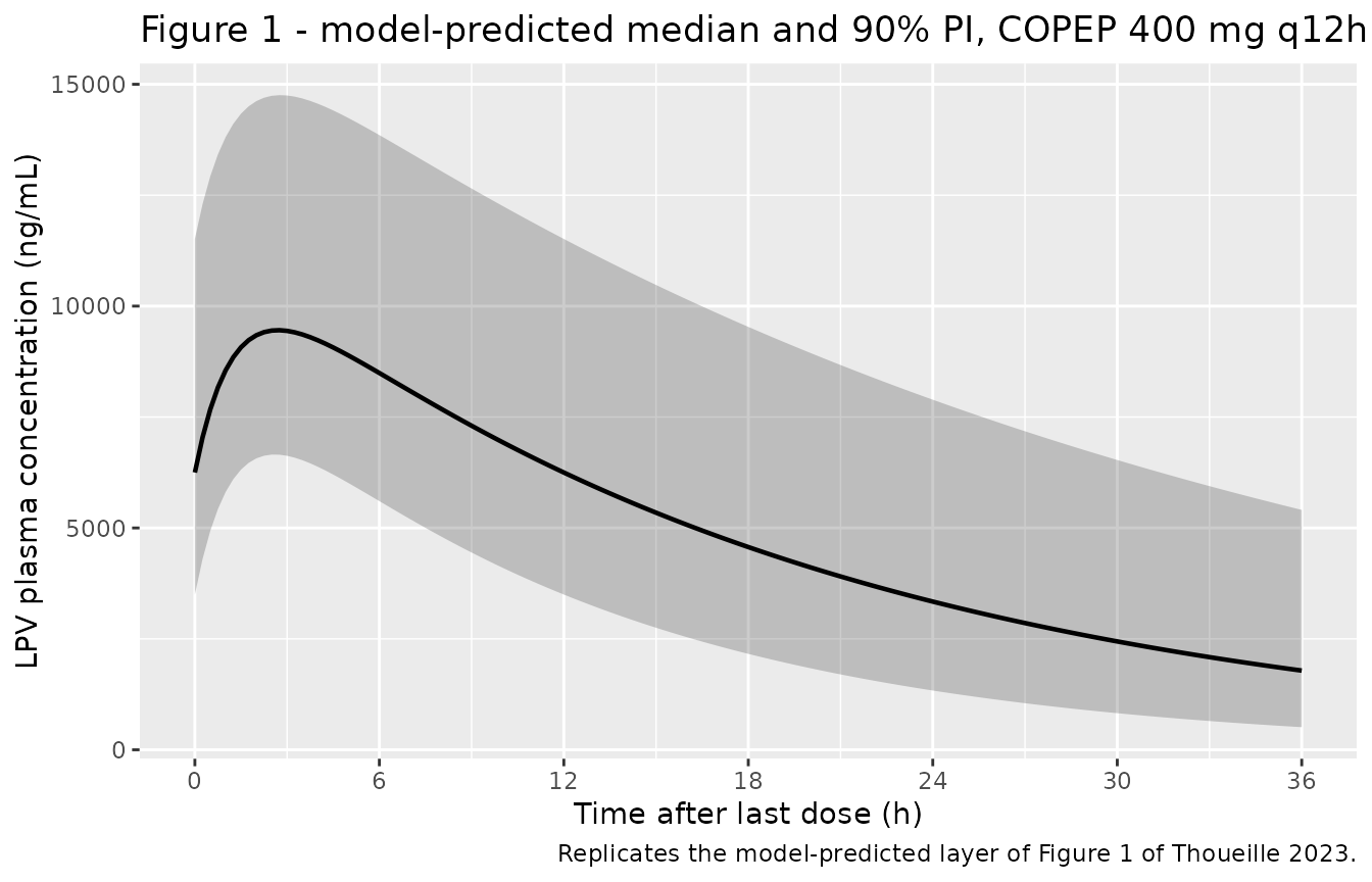
Replicates the model-predicted layer of Figure 1 of Thoueille 2023.
For orientation against the published data cloud: the analysis dataset (Thoueille 2023 Additional file 1) contains 266 lopinavir concentrations spanning 1125-24420 ng/mL with a median of 7714 ng/mL. The simulated steady-state average concentration for a typical 70 kg subject on 400 mg twice daily is 8292 ng/mL, which sits inside that observed spread.
tv_sim |>
  filter(time <= tau) |>
  ggplot(aes(time, Cc * 1000, colour = arm)) +
  geom_line(linewidth = 0.8) +
  scale_x_continuous(breaks = seq(0, 12, by = 2)) +
  labs(x = "Time after dose (h)", y = "LPV plasma concentration (ng/mL)",
       colour = NULL,
       title = "Typical-value steady-state profiles over one 12 h interval")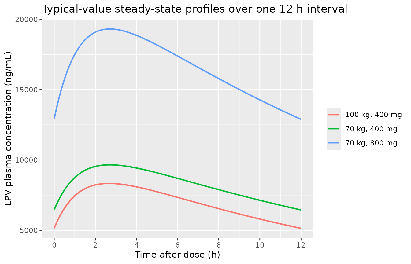
Typical-value steady-state profiles by weight and dose.
PKNCA validation
Steady-state NCA over the 12 h dosing interval (PKNCA recipe 3), plus the terminal half-life estimated from the post-dose decline.
sim_nca <- sim |>
  dplyr::filter(!is.na(Cc)) |>
  dplyr::select(id, time, Cc, cohort)

# Guarantee a time = 0 row per (id, cohort). At steady state the pre-dose
# concentration is the trough, not zero, so take it from the simulation rather
# than substituting 0.
stopifnot(all(sim_nca |> group_by(id) |> summarise(has0 = any(time == 0)) |> pull(has0)))

conc_obj <- PKNCA::PKNCAconc(sim_nca, Cc ~ time | cohort + id,
                             concu = "mg/L", timeu = "h")

dose_df <- events |>
  dplyr::filter(evid == 1) |>
  dplyr::select(id, time, amt, cohort)

dose_obj <- PKNCA::PKNCAdose(dose_df, amt ~ time | cohort + id)

# Terminal half-life is deliberately NOT requested on the steady-state
# interval: inside a single 12 h window the residual absorption tail biases
# lambda-z upward by about 1%. It is estimated instead from the single-dose
# arm below, which is also how the paper derived its published value.
intervals_ss <- data.frame(
  start     = 0,
  end       = tau,
  cmax      = TRUE,
  tmax      = TRUE,
  cmin      = TRUE,
  auclast   = TRUE,
  cav       = TRUE
)

nca_res <- PKNCA::pk.nca(PKNCA::PKNCAdata(conc_obj, dose_obj,
                                          intervals = intervals_ss))

nca_res$result |>
  # PKNCA emits dependency rows for other intervals; filter on the interval
  # bounds as well as the parameter name.
  dplyr::filter(start == 0, end == tau,
                PPTESTCD %in% c("cmax", "tmax", "cmin", "auclast", "cav")) |>
  dplyr::group_by(cohort, PPTESTCD) |>
  dplyr::summarise(median = median(PPORRES, na.rm = TRUE),
                   q05 = quantile(PPORRES, 0.05, na.rm = TRUE),
                   q95 = quantile(PPORRES, 0.95, na.rm = TRUE),
                   .groups = "drop") |>
  tidyr::pivot_wider(names_from = PPTESTCD,
                     values_from = c(median, q05, q95)) |>
  dplyr::select(cohort, dplyr::starts_with("median_")) |>
  dplyr::rename(
    "Cohort"                = cohort,
    "Cmax,ss (mg/L)"        = median_cmax,
    "Tmax,ss (h)"           = median_tmax,
    "Cmin,ss (mg/L)"        = median_cmin,
    "Cavg,ss (mg/L)"        = median_cav,
    "AUC0-tau (mg*h/L)"     = median_auclast
  ) |>
  knitr::kable(digits = 2,
caption = "Median steady-state NCA parameters by simulated cohort (n = 200 each).")| Cohort | AUC0-tau (mg*h/L) | Cavg,ss (mg/L) | Cmax,ss (mg/L) | Cmin,ss (mg/L) | Tmax,ss (h) |
|---|---|---|---|---|---|
| COPEP 400 mg q12h | 97.09 | 8.09 | 9.46 | 6.25 | 2.75 |
| PLWH 400 mg q12h | 102.53 | 8.54 | 9.91 | 6.70 | 2.75 |
| PLWH 800 mg q12h | 202.55 | 16.88 | 19.61 | 13.18 | 2.75 |
Exact identity checks on the typical-value arms
At steady state, AUC0-tau = F * Dose / CL. With no
residual or between-subject variability, this is an exact identity that
the simulation must reproduce, and it turns both the dose
proportionality and the body-weight covariate into strict assertions
rather than eyeball comparisons.
tv_nca_conc <- tv_sim |>
  dplyr::filter(!is.na(Cc)) |>
  dplyr::select(id, time, Cc, arm)

tv_conc_obj <- PKNCA::PKNCAconc(tv_nca_conc, Cc ~ time | arm + id,
                                concu = "mg/L", timeu = "h")

tv_dose_obj <- PKNCA::PKNCAdose(
  tv_events |> dplyr::filter(evid == 1) |> dplyr::select(id, time, amt, arm),
  amt ~ time | arm + id
)

tv_nca <- PKNCA::pk.nca(PKNCA::PKNCAdata(tv_conc_obj, tv_dose_obj,
                                         intervals = intervals_ss))

tv_tbl <- tv_nca$result |>
  dplyr::filter(start == 0, end == tau) |>
  dplyr::select(arm, PPTESTCD, PPORRES) |>
  tidyr::pivot_wider(names_from = PPTESTCD, values_from = PPORRES)

get_val <- function(arm_name, param) {
  tv_tbl[[param]][tv_tbl$arm == arm_name]
}

auc_70_400  <- get_val("70 kg, 400 mg",  "auclast")
auc_70_800  <- get_val("70 kg, 800 mg",  "auclast")
auc_100_400 <- get_val("100 kg, 400 mg", "auclast")

# Identity 1: AUC0-tau = Dose / CL for the 70 kg reference subject, where the
# covariate term is exactly 1 and CL = 4.02 L/h. The 0.5% tolerance absorbs
# linear-trapezoid error on the 0.02 h grid.
auc_expected <- 400 / cl_final
stopifnot(abs(auc_70_400 / auc_expected - 1) < 0.005)

# Identity 2: strict dose proportionality (the model is linear).
stopifnot(abs(auc_70_800 / auc_70_400 - 2) < 1e-3)

# Identity 3: the body-weight effect. A 100 kg subject has CL 19.16% higher than
# a 70 kg subject, so exposure is lower by exactly that factor. This is the
# covariate equation reduced to an exposure ratio.
stopifnot(abs(auc_70_400 / auc_100_400 - (1 + e_wt_cl * (100 - 70) / 70)) < 1e-3)

tibble::tibble(
  Check = c("AUC0-tau (70 kg, 400 mg) vs Dose/CL",
            "AUC0-tau ratio 800 mg / 400 mg",
            "AUC0-tau ratio 70 kg / 100 kg"),
  Simulated = c(auc_70_400, auc_70_800 / auc_70_400, auc_70_400 / auc_100_400),
  Expected  = c(auc_expected, 2, 1 + e_wt_cl * (100 - 70) / 70)
) |>
  knitr::kable(digits = 4,
caption = "Exact steady-state identities (typical-value arms, no variability).")| Check | Simulated | Expected |
|---|---|---|
| AUC0-tau (70 kg, 400 mg) vs Dose/CL | 99.5023 | 99.5025 |
| AUC0-tau ratio 800 mg / 400 mg | 2.0000 | 2.0000 |
| AUC0-tau ratio 70 kg / 100 kg | 1.1916 | 1.1916 |
Comparison against published NCA
Thoueille 2023 reports two model-derived NCA-type quantities, both
computed from the base model. The comparison arm below
therefore uses the base-model parameters (ka = 0.743 1/h,
CL_LPV = 4.05 L/h) at the 70 kg reference weight, where the
final model’s covariate term equals 1, and gives a single dose so that
Tmax and the terminal half-life carry their conventional single-dose
meaning.
base_conc_obj <- PKNCA::PKNCAconc(
  base_sim |> dplyr::filter(!is.na(Cc)) |>
    dplyr::select(id, time, Cc, arm),
  Cc ~ time | arm + id, concu = "mg/L", timeu = "h"
)

base_dose_obj <- PKNCA::PKNCAdose(
  base_events |> dplyr::filter(evid == 1) |>
    dplyr::select(id, time, amt, arm),
  amt ~ time | arm + id
)

intervals_sd <- data.frame(
  start      = 0,
  end        = Inf,
  cmax       = TRUE,
  tmax       = TRUE,
  aucinf.obs = TRUE,
  half.life  = TRUE
)

base_nca <- PKNCA::pk.nca(PKNCA::PKNCAdata(base_conc_obj, base_dose_obj,
                                           intervals = intervals_sd))

published <- tibble::tribble(
  ~arm,                                    ~tmax, ~half.life,
  "Base model, 70 kg, 400 mg single dose",   3.9,       13.5
)

cmp <- nlmixr2lib::ncaComparisonTable(
  simulated     = base_nca,
  reference     = published,
  by            = "arm",
  units         = c(tmax = "h", half.life = "h"),
  tolerance_pct = 20
)

knitr::kable(
  cmp,
  caption = "Simulated vs. published derived quantities (Thoueille 2023 Discussion; Table S1 'In-house' row). * differs from reference by >20%.",
  align   = c("l", "l", "r", "r", "r")
)| NCA parameter | arm | Reference | Simulated | % diff |
|---|---|---|---|---|
| Tmax (h) | Base model, 70 kg, 400 mg single dose | 3.9 | 3.86 | -1.0% |
| t½ (h) | Base model, 70 kg, 400 mg single dose | 13.5 | 13.5 | +0.1% |
base_tbl <- base_nca$result |>
  dplyr::filter(start == 0, is.infinite(end)) |>
  dplyr::select(PPTESTCD, PPORRES) |>
  tidyr::pivot_wider(names_from = PPTESTCD, values_from = PPORRES)

# The base-model half-life must recover the published 13.5 h. The 0.5%
# tolerance absorbs the log-linear regression window PKNCA selects.
stopifnot(abs(base_tbl$half.life / 13.5 - 1) < 0.005)

# AUC0-inf after a single dose is an exact identity: Dose / CL = 400 / 4.05.
# This is the check that catches a stale-parameter solve, which a half-life
# comparison alone does not: the final model's 13.60 h is within 1% of the
# published 13.5 h, but its AUC0-inf of 99.50 is not within 0.5% of 98.77.
stopifnot(abs(base_tbl$aucinf.obs / (400 / 4.05) - 1) < 0.005)

# And Tmax must recover the published 3.9 h to within the 0.02 h grid plus
# rounding (the closed-form value is 3.864 h).
stopifnot(abs(base_tbl$tmax - 3.9) < 0.1)
Both published quantities are reproduced: the simulated half-life and Tmax match the paper’s 13.5 h and 3.9 h, and no row is starred. No parameter was tuned – the base-model values are the ones the paper prints in its Results paragraph and in the Table S1 “In-house” row.
Assumptions and deviations
Between-subject variability scale. Thoueille 2023 Table 2 reports BSV on
CL_LPVas “28.5%” without stating whether the percentage is the standard deviation of the log-normal random effect or the coefficient of variation on the natural scale. It is read here as a natural-scale CV and back-transformed withomega^2 = log(1 + CV^2) = 0.078096, matching the convention used elsewhere in this registry and by the same Lausanne group inCsajka_2004_indinavir. The alternative reading (omega = 0.285, variance 0.081225) differs by 2% on the standard-deviation scale and does not affect any check in this vignette, all of which are typical-value or median-based.Body-weight distributions are simulated, not replayed. Weights are drawn from log-normal distributions whose medians match Thoueille 2023 Table 1 and are clamped to the published ranges. Clamping slightly compresses the tails relative to the real cohort. The participant-level weights are available in Additional file 1 of the paper but are not carried in this package.
Figure 1 is only partially replicated. The published figure is a prediction- and variability-corrected VPC that overlays observed concentrations and their empirical median / PI90 on the model-predicted intervals. Only the model-predicted layer is redrawn here.
The published Tmax and half-life are single-dose base-model quantities. The paper states them in the Discussion having derived them from the base model (
ka0.743,V_LPV78.9,CL_LPV4.05), not from the final covariate model, whose corresponding values are 3.81 h and 13.60 h. They are also single-dose closed forms. The comparison arm therefore overrideslkaandlclat solve time and gives a single 400 mg dose followed for 120 h. Both distinctions matter numerically: at steady state this model peaks at 2.74 h rather than 3.86 h, and a half-life read off a single 12 h steady-state interval is biased upward by about 1% because the absorption tail has not fully decayed.Parameter overrides are passed via
params =, notrxode2::ini(). Once the model has been solved earlier in the vignette,rxSolve()reuses the cached compiled model and silently ignores thetas changed by a subsequentrxode2::ini()call – the modified object reports the new$thetawhile the solve still uses the original values, and rebuilding from a freshreadModelDb()does not help. The base-model arm therefore overrides at solve time and asserts on the solvedclandkacolumns so the substitution cannot fail silently.Bioavailability is not parameterised. Lopinavir was given orally only, so
CL_LPVandV_LPVare apparent (CL/F, V/F). Thoueille 2023 reports no bioavailability term and none is introduced;Fis implicitly 1.The dried-blood-spot to plasma conversion is not part of the model. COPEP concentrations were converted with
C_plasma = C_DBS * F_BP / (1 - HCT)using a protein-binding ratio of 98.5% and a haematocrit assumed at 0.40 for women and 0.45 for men, because haematocrit was not measured. That is a data-preparation step applied before model fitting, so it is documented in theSEXFentry ofcovariatesDataExcludedrather than encoded inmodel(). The authors note in the Discussion that this assumption “may have affected the conversion of lopinavir DBS to plasma concentrations, possibly preventing the identification of other factors influencing lopinavir disposition.”Screened but unretained covariates. Age, sex, height, body mass index, smoking status, and the COPEP-vs-PLWH population indicator were all tested and none was retained; they are recorded in
covariatesDataExcludedfor provenance. The population indicator was tested on every PK parameter, and its rejection is the paper’s central result.Steady state is assumed, not simulated from first dose. Every arm uses
ss = 1withii = 12, matching the paper’s stated assumption. With a 13.6 h half-life against a 12 h interval, a from-zero simulation would not be at steady state within one interval.Ritonavir is not modelled. Lopinavir was administered as LPV/r 400/100 mg; ritonavir acts as a CYP3A4-inhibiting booster and its effect is absorbed into the apparent lopinavir clearance. Thoueille 2023 models lopinavir only.