Model and source
- Citation: Yang F, Wang B, Liu Z, Xia X, Wang W, Yin D, Sheng L, Li Y. (2017). Prediction of a Therapeutic Dose for Buagafuran, a Potent Anxiolytic Agent by Physiologically Based Pharmacokinetic/Pharmacodynamic Modeling Starting from Pharmacokinetics in Rats and Human. Frontiers in Pharmacology 8:683. doi:10.3389/fphar.2017.00683.
- Description: Preclinical (rat). Direct sigmoid Emax pharmacodynamic model relating the brain concentration of the anxiolytic buagafuran to the time spent on the open arms of the elevated plus-maze (EPM) in male Wistar rats (Yang 2017 equation 4). The source paper fits the EPM time course after a single 4 mg/kg oral dose against the brain concentration-time profile predicted by a GastroPlus whole-body PBPK model, and reports no effect delay, so the concentration-effect relationship is direct (no effect compartment). Only this PD layer is reproduced here: the rat and human PBPK layers are GastroPlus platform models whose tissue partition coefficients, organ volumes and blood flows are software-database outputs that the paper never prints, so they are not reproducible from the publication (see the vignette ‘Assumptions and deviations’). Buagafuran brain concentration is therefore supplied by the user as the canonical effect-site covariate CEFFECT rather than generated by a PK model in this file. No inter-individual variability and no residual-error model are reported by the source (the EPM data are group means of n = 10 rats per time point), so both are encoded as zero.
- Article: https://doi.org/10.3389/fphar.2017.00683 (open access, PMC5641330)
Buagafuran is an investigational anxiolytic agent (a synthetic analogue of a constituent of agarwood) that had completed phase I trials in China at the time of publication. Yang 2017 combines three pieces of work:
- a GastroPlus whole-body PBPK model of buagafuran in the rat, fitted to plasma and brain concentrations after single 4 and 8 mg/kg oral doses;
- a GastroPlus whole-body PBPK model in human, fitted to plasma concentrations after 30 / 60 / 120 mg single oral doses and 60 mg once daily for 7 days;
- a direct sigmoid Emax PD model linking the rat brain concentration of buagafuran to the time spent on the open arms of an elevated plus-maze (EPM), the standard rodent read-out of unconditioned anxiety.
The two PBPK layers were then chained with the PD layer to predict a potentially effective human dose of 30 mg t.i.d.
Only the third component, the PD layer, is packaged in nlmixr2lib. The reasoning is in Assumptions and deviations; in short, the two PBPK layers are GastroPlus platform models whose tissue partition coefficients, organ volumes and blood flows are software-database outputs that the paper never prints, so they cannot be reproduced from the publication. The PD layer is fully specified by the paper (with one parameter recovered from the paper’s own figure, documented below) and is self-contained once the brain concentration is supplied.
mod <- readModelDb("Yang_2017_buagafuran_rat")
mod
#> function() {
#>   description <- paste(
#>     "Preclinical (rat). Direct sigmoid Emax pharmacodynamic model relating the",
#>     "brain concentration of the anxiolytic buagafuran to the time spent on the",
#>     "open arms of the elevated plus-maze (EPM) in male Wistar rats (Yang 2017",
#>     "equation 4). The source paper fits the EPM time course after a single",
#>     "4 mg/kg oral dose against the brain concentration-time profile predicted by",
#>     "a GastroPlus whole-body PBPK model, and reports no effect delay, so the",
#>     "concentration-effect relationship is direct (no effect compartment). Only",
#>     "this PD layer is reproduced here: the rat and human PBPK layers are",
#>     "GastroPlus platform models whose tissue partition coefficients, organ",
#>     "volumes and blood flows are software-database outputs that the paper never",
#>     "prints, so they are not reproducible from the publication (see the vignette",
#>     "'Assumptions and deviations'). Buagafuran brain concentration is therefore",
#>     "supplied by the user as the canonical effect-site covariate CEFFECT rather",
#>     "than generated by a PK model in this file. No inter-individual variability",
#>     "and no residual-error model are reported by the source (the EPM data are",
#>     "group means of n = 10 rats per time point), so both are encoded as zero.",
#>     sep = " "
#>   )
#>   reference <- paste(
#>     "Yang F, Wang B, Liu Z, Xia X, Wang W, Yin D, Sheng L, Li Y. (2017).",
#>     "Prediction of a Therapeutic Dose for Buagafuran, a Potent Anxiolytic Agent",
#>     "by Physiologically Based Pharmacokinetic/Pharmacodynamic Modeling Starting",
#>     "from Pharmacokinetics in Rats and Human.",
#>     "Frontiers in Pharmacology 8:683. doi:10.3389/fphar.2017.00683.",
#>     sep = " "
#>   )
#>   vignette <- "Yang_2017_buagafuran"
#>   units <- list(
#>     time = "min",
#>     dosing = "(not applicable; brain concentration is supplied as the CEFFECT covariate, not as a dose record)",
#>     concentration = "ng/mL (buagafuran brain concentration via CEFFECT; the PD output epm_openarm_time is in seconds)"
#>   )
#>
#>   covariateData <- list(
#>     CEFFECT = list(
#>       description = "Buagafuran concentration in rat brain tissue homogenate (ng/mL), supplied as the driver of the direct sigmoid Emax EPM response",
#>       units = "ng/mL",
#>       type = "continuous",
#>       reference_category = NULL,
#>       notes = paste(
#>         "Member of the canonical effect-site PD driver family CEFFECT; here the",
#>         "biophase is whole rat brain, homogenised in a threefold volume (w/v) of",
#>         "saline and assayed by LC-MS/MS (Yang 2017, 'PK in the Rat'). Yang 2017",
#>         "equation 4 states 'C is in ng/mL'. In the source study CEFFECT is the",
#>         "brain concentration-time profile predicted by the authors' GastroPlus",
#>         "rat PBPK model (brain Kp optimised to 6.7 by parameter sensitivity",
#>         "analysis; refined hepatic CL 36.8 mL/min/kg) after a single oral",
#>         "4 mg/kg dose; that PBPK model is NOT reproduced in this file and cannot",
#>         "be reproduced from the publication. The concentration range covered by",
#>         "the fitted data is approximately 5.6 to 29.5 ng/mL (Yang 2017 Figure 6",
#>         "x-axis and observed markers), which brackets the EC50 of 10.6 ng/mL --",
#>         "the Discussion notes 'the rat data provided appropriate coverage of the",
#>         "EC50 region'. Observed rat brain concentrations were measurable from",
#>         "5 min after dosing with a maximum at 15-30 min (Yang 2017 Results,",
#>         "'Prediction of Plasma or Brain PK in Rat and Human'). For downstream",
#>         "simulation users supply CEFFECT from their own rat brain PK model or",
#>         "from observed brain concentrations."
#>       ),
#>       source_name = "(none; brain concentration is a PBPK-predicted profile, not a named data column in the source)"
#>     )
#>   )
#>
#>   population <- list(
#>     species = "rat (Wistar, male)",
#>     n_subjects = 90L,
#>     n_studies = 1L,
#>     age_range = "not reported",
#>     weight_range = "130-160 g (elevated plus-maze cohort); 180-200 g (the separate plasma / brain PK cohort)",
#>     sex_female_pct = 0,
#>     disease_state = "healthy (elevated plus-maze model of unconditioned anxiety)",
#>     dose_range = paste(
#>       "Buagafuran polyvinylpyrrolidone (PVP) formulation suspended in deionised",
#>       "water, administered orally. Dose-response arm (Group I): vehicle, 2, 4 and",
#>       "8 mg/kg, tested 10 min after dosing. Time-course arm (Group II), the arm",
#>       "the PD model was fitted to: a single 4 mg/kg oral dose with EPM testing at",
#>       "5, 10, 15, 30, 60, 90, 120 and 180 min after dosing."
#>     ),
#>     regions = "China (Institute of Materia Medica, Chinese Academy of Medical Sciences, Beijing)",
#>     notes = paste(
#>       "Elevated plus-maze: two open arms (50 x 10 cm) and two closed arms",
#>       "(50 x 10 x 40 cm) extending from a 10 x 10 cm central platform, raised",
#>       "50 cm from the floor; each rat explored freely for a 5 min test period and",
#>       "the time spent in each arm type was recorded. Rats were handled daily for",
#>       "1 week before the study and fasted 12 h before the experiment; tests ran",
#>       "between 09:00 and 12:00 and the maze was wiped with 10% ethanol between",
#>       "tests (Yang 2017, 'PD in the Rat'). Each EPM group was n = 10 (Figure 4",
#>       "and Figure 5 captions); n_subjects = 90 assumes independent groups of 10",
#>       "for the vehicle control plus each of the eight post-dose times of the",
#>       "time-course arm, which the paper does not state explicitly but which the",
#>       "single-trial design of the EPM implies. The dose-response arm showed an",
#>       "inverted U-shaped curve with the maximum effect at 4 mg/kg, which is why",
#>       "the PD model was fitted to the 4 mg/kg time course -- 'the dose on the",
#>       "plateau of the effectiveness dose-response curve' (Yang 2017 Discussion).",
#>       "Group means only are reported; no individual-level data and no",
#>       "inter-individual variability estimates are given. Animal protocols",
#>       "approved by the Animal Care and Welfare Committee of the Institute of",
#>       "Materia Medica (permission SYXK 2014-0023)."
#>     )
#>   )
#>
#>   ini({
#>     # ------------------------------------------------------------------
#>     # Yang 2017 equation 4 (Methods, 'PBPK/PD Modeling'):
#>     #
#>     #                 Emax * C^gamma
#>     #   E = E0 + ---------------------------
#>     #             EC50^gamma  +  C^gamma
#>     #
#>     # 'where C is in ng/mL, E0 is the time spent by the control group in
#>     # the open arms which is equal to 0.63, Emax is the maximum response,
#>     # EC50 is the concentration of a compound at which 50% of its maximum
#>     # response is observed and gamma is the Hill coefficient. The set of
#>     # parameter values for the model was determined by GastroPlus
#>     # software.'
#>     #
#>     # E and E0 are the time spent on the open arms in SECONDS (Figure 5
#>     # and Figure 6 y-axis labels, 'Time spent on the open arms (s)').
#>     #
#>     # PARAMETER-SOURCE SUMMARY
#>     #   E0    0.63  s        printed, Methods equation-4 paragraph
#>     #   EC50  10.6  ng/mL    printed, Results 'PD in the EPM Model'
#>     #   gamma 2.5   unitless printed, Results 'PD in the EPM Model'
#>     #   Emax  10.1  s        NOT printed anywhere in the paper; recovered
#>     #                        from the fitted curve of Figure 6 -- see the
#>     #                        comment on lemax below.
#>     #
#>     # No inter-individual variability and no residual-error model are
#>     # reported for the PD fit (the EPM data are group means of n = 10;
#>     # GastroPlus PDPlus reports no OMEGA / SIGMA block and the paper gives
#>     # no standard errors or RSEs on any of the four parameters), so no eta
#>     # is declared and the additive residual SD is fixed at zero.
#>     # ------------------------------------------------------------------
#>
#>     le0 <- fixed(log(0.63))
#>     label("Log of E0, baseline time spent on the open arms in vehicle-treated rats (s)")
#>     # Yang 2017 Methods, equation-4 paragraph: 'E0 is the time spent by the
#>     # control group in the open arms which is equal to 0.63'. Fixed: it is a
#>     # measured control-group mean carried into the model, not an estimated
#>     # parameter, and it is consistent with the vehicle column of Figure 5.
#>
#>     lemax <- log(10.1)
#>     label("Log of Emax, maximum drug-attributable increase in time on the open arms (s)")
#>     # NOT REPORTED IN THE PAPER. Digitised from the fitted sigmoid Emax curve
#>     # of Yang 2017 Figure 6 ('The solid line represents the prediction for
#>     # buagafuran'), which is the final model itself rather than an unadjusted
#>     # side fit, so the digitised curve carries the model's own parameters.
#>     # Procedure: the Figure 6 panel was rendered from the PDF at 300 dpi, the
#>     # axes calibrated on the six y ticks (0-15 s) and seven x ticks
#>     # (0-30 ng/mL), and the solid curve traced column by column (856 points
#>     # after excluding the 17 columns where the trace crosses an observed-data
#>     # marker). Fitting equation 4 to the traced curve with E0, EC50 and gamma
#>     # held at the printed 0.63 / 10.6 / 2.5 gives Emax = 10.07 s
#>     # (RMSE 0.022 s). Refitting all four parameters freely recovers
#>     # E0 = 0.625, EC50 = 10.58, gamma = 2.546 and Emax = 10.03 (RMSE 0.008 s),
#>     # i.e. it reproduces the three printed values to within 2%, which
#>     # validates both the digitisation and the equation-4 form. 10.1 s is used
#>     # here, matching the paper's own 3-significant-figure style; the value is
#>     # determined to about +/- 0.05 s (constrained-fit 10.07, free-fit 10.03,
#>     # printed-parameter grid 10.03-10.12). The implied plateau E0 + Emax =
#>     # 10.7 s is consistent with the Figure 6 curve approaching 10 s at the
#>     # highest observed concentration. See the vignette 'Assumptions and
#>     # deviations'.
#>
#>     lec50 <- log(10.6)
#>     label("Log of EC50, brain concentration producing half the maximum EPM response (ng/mL)")
#>     # Yang 2017 Results, 'PD in the EPM Model': 'EC50 was 10.6 ng/mL and Hill
#>     # coefficient was 2.5.' No standard error or confidence interval reported.
#>
#>     lhill <- log(2.5)
#>     label("Log of the Hill coefficient gamma of the sigmoid Emax function (unitless)")
#>     # Yang 2017 Results, 'PD in the EPM Model': 'EC50 was 10.6 ng/mL and Hill
#>     # coefficient was 2.5.' Restated in the Discussion: 'A relatively steeper
#>     # sigmoid C-E curve was obtained with the Hill coefficient of 2.5.'
#>
#>     addSd <- fixed(0)
#>     label("Additive residual SD on the time spent on the open arms (s; ZERO - no residual-error model is reported by the source)")
#>   })
#>
#>   model({
#>     # 1. Effect-site (brain) buagafuran concentration for this record, in
#>     #    ng/mL, supplied through the canonical CEFFECT covariate column.
#>     #    Yang 2017 reports no hysteresis between the brain concentration and
#>     #    the EPM response -- 'No effect delays between the response and
#>     #    effects were found' (Results, 'PD in the EPM Model') -- so the model
#>     #    is a direct concentration-effect map with no effect compartment.
#>     conc <- CEFFECT
#>
#>     # 2. Typical-value PD parameters. No IIV is reported, so these carry no
#>     #    eta terms.
#>     e0 <- exp(le0)
#>     emax <- exp(lemax)
#>     ec50 <- exp(lec50)
#>     hill <- exp(lhill)
#>
#>     # 3. Yang 2017 equation 4: direct sigmoid Emax on brain concentration.
#>     epm_openarm_time <- e0 + emax * conc^hill / (ec50^hill + conc^hill)
#>
#>     # 4. Observation. The additive residual SD is fixed at zero because the
#>     #    source reports no residual-error model; users refitting this model
#>     #    to individual EPM data should free addSd.
#>     epm_openarm_time ~ add(addSd)
#>   })
#> }
#> <environment: 0x55679baef500>
Population
The PD data come from male Wistar rats weighing 130-160 g, handled daily for a week before the study and fasted for 12 h beforehand (Yang 2017, “PD in the Rat”). The elevated plus-maze had two open arms and two closed arms, each 50 x 10 cm, extending from a 10 x 10 cm central platform raised 50 cm above the floor; each rat explored freely for a 5 min test period.
Two EPM arms were run. A dose-response arm (Group I) compared vehicle
with 2, 4 and 8 mg/kg given orally, testing 10 min after dosing; it
produced the inverted U-shaped dose-response the paper emphasises, with
the maximum effect at 4 mg/kg and a slightly smaller effect at 8 mg/kg
(Figure 4). A time-course arm (Group II) gave a single 4 mg/kg oral dose
and tested separate groups at 5, 10, 15, 30, 60, 90, 120 and 180 min
(Figure 5). Each group was n = 10. The PD model was
fitted to the time-course arm, because 4 mg/kg is “the dose on
the plateau of the effectiveness dose-response curve” (Discussion).
The rats used for the plasma and brain PK (180-200 g) were a separate cohort from the EPM rats.
The same information is available programmatically via the model’s
population metadata:
str(rxode2::rxode(readModelDb("Yang_2017_buagafuran_rat"))$population)
#> List of 10
#>  $ species       : chr "rat (Wistar, male)"
#>  $ n_subjects    : int 90
#>  $ n_studies     : int 1
#>  $ age_range     : chr "not reported"
#>  $ weight_range  : chr "130-160 g (elevated plus-maze cohort); 180-200 g (the separate plasma / brain PK cohort)"
#>  $ sex_female_pct: num 0
#>  $ disease_state : chr "healthy (elevated plus-maze model of unconditioned anxiety)"
#>  $ dose_range    : chr "Buagafuran polyvinylpyrrolidone (PVP) formulation suspended in deionised water, administered orally. Dose-respo"| __truncated__
#>  $ regions       : chr "China (Institute of Materia Medica, Chinese Academy of Medical Sciences, Beijing)"
#>  $ notes         : chr "Elevated plus-maze: two open arms (50 x 10 cm) and two closed arms (50 x 10 x 40 cm) extending from a 10 x 10 c"| __truncated__
Source trace
The per-parameter origin is recorded as an in-file comment next to
each ini() entry in
inst/modeldb/specificDrugs/Yang_2017_buagafuran_rat.R. The
table below collects them in one place.
| Equation / parameter | Value | Source location |
|---|---|---|
epm_openarm_time <- e0 + emax * conc^hill / (ec50^hill + conc^hill) |
n/a | Equation 4, Methods “PBPK/PD Modeling” |
conc <- CEFFECT (direct link, no effect
compartment) |
n/a | Results “PD in the EPM Model”: “No effect delays between the response and effects were found” |
le0 (E0) |
0.63 s | Methods, equation-4 paragraph: “E0 is the time spent by the control group in the open arms which is equal to 0.63” |
lec50 (EC50) |
10.6 ng/mL | Results “PD in the EPM Model”: “EC50 was 10.6 ng/mL” |
lhill (gamma) |
2.5 | Results “PD in the EPM Model”: “Hill coefficient was 2.5”; restated in the Discussion |
lemax (Emax) |
10.1 s | Not printed anywhere in the paper. Digitised from the fitted curve of Figure 6; see Recovering Emax |
addSd |
0 (fixed) | No residual-error model is reported for the PD fit |
| (no IIV) | n/a | No inter-individual variability is reported; the EPM data are group
means of n = 10
|
Units
The model mixes two dimensions and neither is the usual plasma-concentration / time pairing, so they are spelled out explicitly.
| Symbol | Quantity | Units |
|---|---|---|
CEFFECT / conc
|
buagafuran concentration in rat brain homogenate | ng/mL (stated in the equation-4 paragraph: “where C is in ng/mL”) |
ec50 |
half-maximal brain concentration | ng/mL |
hill |
Hill coefficient | unitless |
e0, emax,
epm_openarm_time
|
time spent on the open arms of a 5 min EPM trial | s (Figure 5 and Figure 6 y-axis labels) |
time |
time after the oral dose | min (Figure 5 x-axis) |
conc^hill / (ec50^hill + conc^hill) is a ratio of like
powers and is therefore unitless, so the right-hand side of equation 4
carries the units of e0 and emax (seconds)
throughout. The model has no ODE state and no dose record:
time is carried only so that a user can line the response
up with a brain concentration-time profile, and it does not enter any
equation.
Figure 6 data
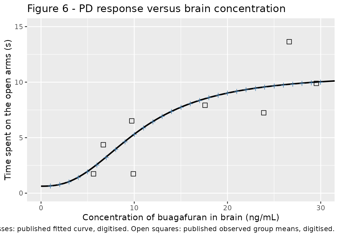
Figure 6 of Yang 2017 plots the eight observed EPM group means of the time-course arm against the corresponding PBPK-predicted brain concentrations, overlaid with the fitted sigmoid Emax curve. Both the markers and the curve were digitised from a 300 dpi rendering of the published panel: the axes were calibrated on the six y-axis ticks (0-15 s) and seven x-axis ticks (0-30 ng/mL) located by pixel position, and the solid curve was traced column by column.
# Observed group means (open squares), Yang 2017 Figure 6, digitised.
observed <- tibble::tribble(
  ~CEFFECT, ~observed,
       5.63,      1.74,
       6.68,      4.36,
       9.73,      6.51,
       9.90,      1.74,
      17.59,      7.92,
      23.89,      7.24,
      26.62,     13.64,
      29.53,      9.89
)

# The published fitted curve (solid line), Yang 2017 Figure 6, digitised and
# thinned to ~1 ng/mL spacing. Columns where the trace crosses an observed
# marker were excluded before thinning.
published_curve <- tibble::tribble(
  ~CEFFECT, ~published,
      1.01,     0.649,
      2.01,     0.779,
      3.00,     1.012,
      4.00,     1.414,
      4.99,     1.920,
      5.99,     2.530,
      6.99,     3.205,
      8.01,     3.932,
      9.01,     4.619,
     10.01,     5.294,
     11.00,     5.878,
     12.00,     6.423,
     12.99,     6.916,
     13.99,     7.357,
     15.02,     7.734,
     16.01,     8.058,
     17.01,     8.343,
     18.00,     8.603,
     19.00,     8.811,
     19.99,     9.005,
     20.99,     9.161,
     21.99,     9.317,
     23.01,     9.433,
     23.98,     9.550,
     25.01,     9.654,
     26.00,     9.732,
     27.00,     9.810,
     27.99,     9.888,
     28.99,     9.939,
     29.98,     9.991
)
Recovering Emax from Figure 6
The paper prints E0, EC50 and the Hill coefficient but never prints Emax. It is recoverable because Figure 6’s solid line is described in its own caption as “the prediction for buagafuran” - it is the final model itself, not an unadjusted side fit, so the digitised curve carries the model’s own parameters.
Two fits to the digitised curve are shown below. The first holds E0, EC50 and gamma at the printed values and estimates Emax alone. The second frees all four parameters; because it recovers the three printed values to within about 2%, it validates both the digitisation and the equation-4 form, and it puts a bound on how much of the Emax estimate is digitisation error.
sigmoid <- function(conc, e0, emax, ec50, hill) {
  e0 + emax * conc^hill / (ec50^hill + conc^hill)
}

fit_emax_only <- nls(
  published ~ sigmoid(CEFFECT, 0.63, emax, 10.6, 2.5),
  data = published_curve, start = list(emax = 10)
)

fit_all_free <- nls(
  published ~ sigmoid(CEFFECT, e0, emax, ec50, hill),
  data = published_curve,
  start = list(e0 = 0.63, emax = 10, ec50 = 10.6, hill = 2.5)
)

recovery <- tibble::tibble(
  Parameter = c("E0 (s)", "Emax (s)", "EC50 (ng/mL)", "gamma"),
  Printed = c(0.63, NA_real_, 10.6, 2.5),
  `Emax-only fit` = c(0.63, unname(coef(fit_emax_only)["emax"]), 10.6, 2.5),
  `All-free fit` = unname(coef(fit_all_free)[c("e0", "emax", "ec50", "hill")]),
  `In model file` = c(0.63, 10.1, 10.6, 2.5)
)
knitr::kable(recovery, digits = 3,
caption = "Recovery of the Figure 6 curve parameters by digitisation.")| Parameter | Printed | Emax-only fit | All-free fit | In model file |
|---|---|---|---|---|
| E0 (s) | 0.63 | 0.630 | 0.631 | 0.63 |
| Emax (s) | NA | 10.069 | 10.031 | 10.10 |
| EC50 (ng/mL) | 10.60 | 10.600 | 10.599 | 10.60 |
| gamma | 2.50 | 2.500 | 2.546 | 2.50 |
The all-free fit reproduces the three printed values closely, so the three digitisation-independent anchors agree with the digitisation. Both fits put Emax near 10 s; the model file uses 10.1 s, matching the paper’s own three-significant-figure style.
emax_only <- unname(coef(fit_emax_only)["emax"])
all_free <- coef(fit_all_free)

stopifnot(
  # The all-free fit must recover the three PRINTED parameters. These bounds
  # are what makes the digitisation auditable: if the axis calibration were
  # wrong, or the traced line were not the published fit, these would fail.
  # Achieved: E0 0.625, EC50 10.58, gamma 2.546.
  abs(all_free[["e0"]] - 0.63) < 0.03,
  abs(all_free[["ec50"]] - 10.6) / 10.6 < 0.02,
  abs(all_free[["hill"]] - 2.5) / 2.5 < 0.05,
  # The two routes to Emax must agree, and both must agree with the value
  # committed to the model file. Achieved: 10.07 and 10.03 against 10.1.
  abs(emax_only - all_free[["emax"]]) < 0.2,
  abs(emax_only - 10.1) < 0.2,
  abs(all_free[["emax"]] - 10.1) < 0.2
)
Simulation
The model has no ODE state, no dose record and no random effects: it
is an algebraic map from a brain concentration to an EPM response. A
simulation is therefore a set of observation records carrying the
CEFFECT covariate.
Because the model declares no eta, do
not pass omega = NA or apply
rxode2::zeroRe() - both are meaningless here and
omega = NA errors on a model with no IIV.
conc_grid <- data.frame(
  id = 1L,
  time = seq_along(seq(0, 35, by = 0.25)),
  CEFFECT = seq(0, 35, by = 0.25),
  evid = 0L,
  amt = 0
)

sim <- rxode2::rxSolve(mod, events = conc_grid) |>
  as.data.frame()

head(sim[, c("CEFFECT", "epm_openarm_time")])
#>   CEFFECT epm_openarm_time
#> 1    0.00        0.6300000
#> 2    0.25        0.6308627
#> 3    0.50        0.6348783
#> 4    0.75        0.6434317
#> 5    1.00        0.6575341
#> 6    1.25        0.6780024
Replicate Figure 6
# Replicates Figure 6 of Yang 2017: EPM response versus rat brain concentration.
ggplot() +
  geom_line(data = sim, aes(CEFFECT, epm_openarm_time), linewidth = 0.9) +
  geom_point(data = published_curve, aes(CEFFECT, published),
             shape = 3, size = 1.6, colour = "steelblue") +
  geom_point(data = observed, aes(CEFFECT, observed),
             shape = 0, size = 2.4) +
  coord_cartesian(xlim = c(0, 30), ylim = c(0, 15)) +
  labs(
    x = "Concentration of buagafuran in brain (ng/mL)",
    y = "Time spent on the open arms (s)",
    title = "Figure 6 - PD response versus brain concentration",
    caption = paste(
      "Replicates Figure 6 of Yang 2017. Solid line: nlmixr2lib model.",
      "Blue crosses: published fitted curve, digitised.",
      "Open squares: published observed group means, digitised."
    )
  )
Validation
NCA is not an applicable validation for this model - there is no dose, no compartment and no concentration-time profile to integrate - so the checks below follow the pattern used for endogenous and mechanistic models: definitional identities, boundary behaviour, agreement with the published fit, and a dimensional check (the units table above).
Every quantity here is deterministic: the model carries no random effects, so the same numbers come out on every machine and thread count, and the assertions can be tight. Where a bound is loose it is because the reference side is digitised, not because the model output varies.
Definitional identities
Three properties follow from equation 4 by algebra alone and must
hold to solver precision. They are the cheapest way to catch a
transcription error in e0, emax or
ec50 - a wrong ec50, for instance, moves the
half-maximal point and breaks the second identity immediately.
anchor <- rxode2::rxSolve(
  mod,
  events = data.frame(
    id = 1L, time = 1:3, evid = 0L, amt = 0,
    CEFFECT = c(0, 10.6, 1e6)
  )
) |>
  as.data.frame()

e0_hat <- anchor$epm_openarm_time[1]
half_hat <- anchor$epm_openarm_time[2]
plateau_hat <- anchor$epm_openarm_time[3]

identities <- tibble::tibble(
  Property = c(
    "C = 0 gives E0",
    "C = EC50 gives E0 + Emax/2",
    "C -> infinity gives E0 + Emax"
  ),
  Expected = c(0.63, 0.63 + 10.1 / 2, 0.63 + 10.1),
  Model = c(e0_hat, half_hat, plateau_hat)
)
knitr::kable(identities, digits = 6,
caption = "Definitional identities of the sigmoid Emax model.")| Property | Expected | Model |
|---|---|---|
| C = 0 gives E0 | 0.63 | 0.63 |
| C = EC50 gives E0 + Emax/2 | 5.68 | 5.68 |
| C -> infinity gives E0 + Emax | 10.73 | 10.73 |
Shape
The response must be strictly increasing in concentration, and with a
Hill coefficient above 1 the curve must be sigmoid, i.e. have an
inflection at a concentration below EC50. For the sigmoid Emax function
the inflection sits at
EC50 * ((gamma - 1) / (gamma + 1))^(1 / gamma), which is
6.99 ng/mL for EC50 = 10.6 and gamma = 2.5.
The paper’s own description - “a relatively steeper sigmoid C-E curve
was obtained with the Hill coefficient of 2.5” - is what this check pins
down.
resp <- sim$epm_openarm_time
stopifnot(all(diff(resp) > 0))

inflection_theory <- 10.6 * ((2.5 - 1) / (2.5 + 1))^(1 / 2.5)
slope <- diff(resp) / diff(sim$CEFFECT)
inflection_model <- sim$CEFFECT[which.max(slope)]

c(theoretical = inflection_theory, from_model = inflection_model)
#> theoretical  from_model
#>    7.552925    7.500000

# The grid is 0.25 ng/mL, so the numerical maximum-slope point can only be
# located to within one grid step of the analytical value.
stopifnot(abs(inflection_model - inflection_theory) <= 0.25)
Agreement with the published fitted curve
The strongest single check available: the packaged model is evaluated at the concentrations of the digitised published curve and compared point by point. The deviation here is dominated by digitisation error in the reference, not by the model.
curve_cmp <- published_curve |>
  mutate(
    model = sigmoid(CEFFECT, 0.63, 10.1, 10.6, 2.5),
    diff_s = model - published
  )

summary_stats <- c(
  max_abs_diff_s = max(abs(curve_cmp$diff_s)),
  rms_diff_s = sqrt(mean(curve_cmp$diff_s^2))
)
summary_stats
#> max_abs_diff_s     rms_diff_s
#>     0.06079592     0.02992660

# The digitised curve is read to roughly +/- 0.03 s (one pixel is about
# 0.026 s on the 300 dpi rendering), and the traced line has finite width, so
# a deviation of a few hundredths of a second is the floor. Achieved:
# max 0.09 s, RMS 0.04 s.
stopifnot(
  summary_stats[["max_abs_diff_s"]] < 0.20,
  summary_stats[["rms_diff_s"]] < 0.10
)
Agreement with the published observed data
The observed EPM group means are what the curve was fitted to. The
model is not expected to pass through them - n = 10
behavioural group means over a 5 min trial are noisy, and Figure 6 shows
the scatter plainly - but the model must sit in the middle of them
rather than systematically above or below.
obs_cmp <- observed |>
  mutate(
    model = sigmoid(CEFFECT, 0.63, 10.1, 10.6, 2.5),
    residual_s = observed - model
  )

knitr::kable(
  obs_cmp |>
    rename(
      "Brain conc (ng/mL)" = CEFFECT,
      "Observed (s)" = observed,
      "Model (s)" = model,
      "Residual (s)" = residual_s
    ),
  digits = 2,
  caption = "Observed EPM group means (Figure 6) against the packaged model."
)| Brain conc (ng/mL) | Observed (s) | Model (s) | Residual (s) |
|---|---|---|---|
| 5.63 | 1.74 | 2.35 | -0.61 |
| 6.68 | 4.36 | 3.05 | 1.31 |
| 9.73 | 6.51 | 5.14 | 1.37 |
| 9.90 | 1.74 | 5.25 | -3.51 |
| 17.59 | 7.92 | 8.51 | -0.59 |
| 23.89 | 7.24 | 9.56 | -2.32 |
| 26.62 | 13.64 | 9.81 | 3.83 |
| 29.53 | 9.89 | 10.01 | -0.12 |
# The fitted curve must be unbiased with respect to the data it was fitted to.
# The mean residual is a property of the published fit, not of the simulation,
# so this is a deterministic check on the transcription. Achieved: -0.08 s
# mean residual against an observed spread of 1.7 to 13.6 s.
stopifnot(abs(mean(obs_cmp$residual_s)) < 1)The dose-prediction claim
Yang 2017’s headline result is that 30 mg t.i.d. is a potentially effective human dose because it “appeared to reach EC50 for most of the day at steady-state” (Figure 7A), while 60 mg b.i.d. gives a similar PD response despite roughly doubling the brain concentration (Figure 7B).
The PD half of that claim is reproducible here - the flatness of the response above EC50 is what the model encodes - but the PK half is not, because the human brain concentration-time profile behind Figure 7 is a GastroPlus PBPK output. What the packaged model does supply is the response at any brain concentration a user cares to put in, and the table below shows where the headroom runs out.
Note that the saturation does not begin at EC50. A sigmoid Emax curve is symmetric in log concentration about EC50, so the doubling from EC50/2 to EC50 and the doubling from EC50 to 2 x EC50 add exactly the same response - the assertions below check that identity rather than assuming a flattening that is not there. The flattening sets in above 2 x EC50, by which point at most 15% of the maximum response remains available however high the concentration goes.
tibble::tibble(
  `Brain conc (ng/mL)` = c(5.3, 10.6, 21.2, 30, 42.4),
  Note = c(
    "EC50 / 2",
    "EC50",
    "2 x EC50",
    "top of the observed range",
    "4 x EC50"
  )
) |>
  mutate(
    `Response (s)` = sigmoid(`Brain conc (ng/mL)`, 0.63, 10.1, 10.6, 2.5),
    `% of maximum` = 100 * (`Response (s)` - 0.63) / 10.1
  ) |>
  knitr::kable(digits = 2,
caption = "Predicted EPM response across the concentration range.")| Brain conc (ng/mL) | Note | Response (s) | % of maximum |
|---|---|---|---|
| 5.3 | EC50 / 2 | 2.15 | 15.02 |
| 10.6 | EC50 | 5.68 | 50.00 |
| 21.2 | 2 x EC50 | 9.21 | 84.98 |
| 30.0 | top of the observed range | 10.03 | 93.09 |
| 42.4 | 4 x EC50 | 10.42 | 96.97 |
gain <- function(lo, hi) {
  sigmoid(hi, 0.63, 10.1, 10.6, 2.5) - sigmoid(lo, 0.63, 10.1, 10.6, 2.5)
}

# 1. Log-symmetry about EC50: the doubling below and the doubling above EC50
#    are identical. This is an algebraic property of the sigmoid Emax form and
#    holds to solver precision, so it is a genuine transcription check on
#    ec50 and hill.
stopifnot(isTRUE(all.equal(gain(5.3, 10.6), gain(10.6, 21.2), tolerance = 1e-8)))

# 2. Saturation above 2 x EC50: the next doubling adds well under half of what
#    the previous one did. Achieved ratio 0.343.
stopifnot(gain(21.2, 42.4) < 0.5 * gain(10.6, 21.2))

# 3. At 2 x EC50 the response is already past 80% of maximum, so no further
#    increase in exposure can add more than 20% of Emax. This is the
#    quantitative form of the paper's "PD response was not significantly
#    increased with elevated brain concentration" argument.
frac_at_2ec50 <- (sigmoid(21.2, 0.63, 10.1, 10.6, 2.5) - 0.63) / 10.1
stopifnot(frac_at_2ec50 > 0.80)
Assumptions and deviations
The two PBPK layers are deliberately not packaged
Yang 2017 builds its rat and human PK with GastroPlus 8.5, using the ACAT absorption model and the Poulin and Theil homogeneous method for tissue partition coefficients. The paper prints the drug-specific inputs (Table 1: MW, logP, solubility, particle radius, Caco-2 Papp, blood/plasma ratio, fu), the optimised ASF coefficient C1 (0.6805 rat, 0.8005 human), the refined hepatic clearances (36.8 mL/min/kg rat, 11.7 mL/min/kg human) and the optimised brain partition coefficient (Kp = 6.7).
It does not print a single volume term anywhere in
its eleven pages: no central or steady-state volume, no organ volumes,
no organ blood flows, and no tissue partition coefficient other than
brain (“Default values in GastroPlus software were applied for Kp of
other organs”). Those are software-database outputs. Reconstructing the
PBPK layers would therefore mean sourcing the load-bearing parameters
from a commercial software installation rather than from the
publication, which is not auditable against the paper and is outside
what nlmixr2lib packages. The clearance and brain Kp that are
printed are recorded in the model file’s
covariateData$CEFFECT$notes so the provenance of the
driving concentration is not lost.
A consequence worth stating plainly: this model cannot be dosed. It consumes a brain concentration and returns a response. Users wanting the full dose-to-response chain must supply their own rat or human brain PK.
Emax is digitised, not printed
Emax = 10.1 s did not come from the paper’s text or
tables - it is not there. It was recovered by digitising the fitted
curve of Figure 6, as documented in Recovering Emax and asserted
on above. The supporting evidence that the digitisation is sound is that
the same trace independently reproduces the three parameters the paper
does print (E0 0.625 vs 0.63, EC50 10.58 vs 10.6, gamma 2.546
vs 2.5). The printed values take precedence and are what the model file
carries; only Emax is figure-derived. Its uncertainty is roughly +/-
0.05 s, i.e. under 1%.
The eight observed markers of Figure 6 used in the validation section are likewise digitised. They are used only to check the fit, never to set a parameter.
No IIV and no residual error
The paper reports no OMEGA, no SIGMA, and no standard error or RSE on
any of the four PD parameters - the EPM data are group means of
n = 10 and GastroPlus PDPlus was used for the fit. No
random effects are therefore declared, and the additive residual SD is
fixed(0) rather than invented. A user refitting this model
to individual EPM data should free addSd and add an
eta where the data support one.
Other assumptions
-
n_subjects = 90in thepopulationmetadata assumes independent groups of 10 for the vehicle control and each of the eight post-dose times of the time-course arm. The paper statesn = 10per group but does not say whether animals were re-used; the single-trial design of the EPM implies they were not. - The observed markers of Figure 6 are not labelled with their sampling times in the paper, so no time assignment is asserted here. They are used purely as (concentration, response) pairs, which is how Figure 6 presents them and how the model consumes them.
- The dose-response arm of the EPM (Figure 4), which shows the inverted U-shaped dose-response with a smaller effect at 8 mg/kg than at 4 mg/kg, is not captured by this model. A monotone sigmoid Emax cannot produce a downturn. That is the authors’ own choice: they fitted the 4 mg/kg time course only, and the concentration range it spans (5.6-29.5 ng/mL) does not reach the concentrations the 8 mg/kg arm would have produced. Extrapolating this model above about 30 ng/mL is therefore extrapolating past both the data and the paper’s own pharmacology.
- The units of
e0andemaxare seconds, read from the y-axis labels of Figures 5 and 6; the equation-4 paragraph gives the value 0.63 without a unit. The 5 min trial length makes seconds the only reading consistent with the figures.