Model and source
Citation: Zou Y, Ren J, Lei H, Chen G, Li C, He X, Hu Y, Liu X. Population pharmacokinetic modeling and Monte Carlo simulation to optimize meropenem dosing in patients with severe postoperative infections. Front Pharmacol. 2026;17:1778552. doi:10.3389/fphar.2026.1778552.
Description: One-compartment IV population PK model for meropenem in 44 Chinese adults with severe postoperative infections receiving therapeutic drug monitoring in a general ICU (Zou 2026). Postoperative Cockcroft-Gault creatinine clearance acts as a power covariate on CL, centred at the cohort mean of 47.7 mL/min. Inter-individual variability on CL and Vc is strongly correlated (rho = 0.94). Residual error is additive; see the vignette Errata for the reconciliation of Table 2’s residual-error row, which reports a variance where the bootstrap column reports a standard deviation.
Zou and colleagues developed a one-compartment population PK model for meropenem in 44 adults with severe postoperative infections managed in a general ICU, then used Monte Carlo simulation to derive renal-function- and MIC-stratified dosing recommendations. This vignette reproduces the structural model, confirms the packaged encoding against a closed-form steady-state solution, and reproduces the published probability-of-target-attainment (PTA) recommendations of the paper’s Table 3.
Population
Forty-four adults (31 male, 70.45%) contributed 135 plasma meropenem concentrations. All were postoperative patients with severe infection requiring meropenem for more than three days; 93.18% were classified as critically ill and 15.91% were receiving haemodialysis. The most common presentation was intra-abdominal infection combined with hospital-acquired pneumonia (47.73%). Patients received 1.0 g meropenem every 8 h as a prolonged infusion over 2 h or 2.5 h, with TDM-guided adjustment permitted; samples were drawn at steady state after at least four consecutive doses (Zou 2026 Table 1, Sections 2.1-2.3).
Cockcroft-Gault creatinine clearance had a cohort mean of 47.7 mL/min and ranged from 11.9 to 136 mL/min (Table 1). Observed meropenem concentrations had a mean of 16.183 mg/L and ranged from 0.477 to 71.507 mg/L.
The same information is available programmatically via the model’s
population metadata
(readModelDb("Zou_2026_meropenem")()$population).
Source trace
The per-parameter origin is recorded as an in-file comment next to
each ini() entry in
inst/modeldb/specificDrugs/Zou_2026_meropenem.R. The table
below collects them in one place for review.
| Equation / parameter | Value | Source location |
|---|---|---|
lcl (typical CL) |
6.472 L/h | Table 2, “Final model” column, CL row (RSE 8.53%) |
lvc (typical Vc) |
26.69 L | Table 2, “Final model” column, Vc row (RSE 13.55%) |
e_crcl_cl |
0.3834 | Table 2, “CRCL on CL” row (RSE 16.54%) |
crcl_ref_cl |
47.7 mL/min | Section 3.2 covariate equation denominator; equals the Table 1 cohort mean CRCL |
var(etalcl) |
0.494^2 = 0.244036 | Table 2, omega-CL = 49.4%, footnote “square root of inter-individual variance” |
var(etalvc) |
0.8199^2 = 0.672236 | Table 2, omega-Vc = 81.99%, same footnote |
cov(etalcl, etalvc) |
0.94 x 0.494 x 0.8199 = 0.380727 | Table 2, omega-CL*Vc row, rho = 0.94 |
addSd |
sqrt(17.4) = 4.17 mg/L | Table 2 residual-error row (see Errata: the column reports a variance) |
CL = 6.472 * (CrCL/47.7)^0.3834 * exp(eta_CL) |
n/a | Section 3.2, displayed covariate equation |
Vc = 26.69 * exp(eta_Vc) |
n/a | Section 3.2, displayed covariate equation |
d/dt(central) = -kel * central |
n/a | Section 3.2, “one-compartment model with linear elimination” |
Structural verification
Before any cohort simulation, the packaged encoding is checked against results that do not depend on a random draw.
Covariate relation
The individual clearance returned by the solver must equal the published covariate equation exactly.
mod <- readModelDb("Zou_2026_meropenem")

crcl_grid <- c(11.9, 25, 47.7, 90, 136)
ev_cov <- rxode2::et(amt = 1000, dur = 2, cmt = "central") |>
  rxode2::et(seq(0, 8, by = 1), cmt = "central") |>
  as.data.frame()
ev_cov <- do.call(rbind, lapply(seq_along(crcl_grid), function(i) {
  x <- ev_cov; x$id <- i; x$CRCL <- crcl_grid[i]; x
}))

# zeroRe() removes IIV so cl is the typical value at each CRCL.
cov_chk <- rxode2::rxSolve(rxode2::zeroRe(mod), ev_cov, returnType = "data.frame") |>
  dplyr::group_by(id, CRCL) |>
  dplyr::summarise(cl_solved = mean(cl), .groups = "drop") |>
  dplyr::mutate(cl_published = 6.472 * (CRCL / 47.7)^0.3834,
                rel_err = abs(cl_solved / cl_published - 1))
#> ℹ omega/sigma items treated as zero: 'etalcl', 'etalvc'
#> Warning: multi-subject simulation without without 'omega'

knitr::kable(
  cov_chk |>
    dplyr::rename("CRCL (mL/min)" = CRCL,
                  "CL solved (L/h)" = cl_solved,
                  "CL published equation (L/h)" = cl_published,
                  "Relative error" = rel_err) |>
    dplyr::select(-id),
  digits = c(0, 1, 4, 4, 12),
  caption = "Solved individual clearance vs the Section 3.2 covariate equation."
)| CRCL (mL/min) | CL solved (L/h) | CL published equation (L/h) | Relative error |
|---|---|---|---|
| 12 | 3.8 | 3.8007 | 0 |
| 25 | 5.1 | 5.0520 | 0 |
| 48 | 6.5 | 6.4720 | 0 |
| 90 | 8.3 | 8.2556 | 0 |
| 136 | 9.7 | 9.6715 | 0 |
# Deterministic: same equation, no random draw. A tight bound is correct here.
stopifnot(max(cov_chk$rel_err) < 1e-10)
At the reference CRCL of 47.7 mL/min the clearance returns exactly the published typical value of 6.472 L/h, confirming both the centring constant and the exponent.
Closed-form steady-state solution
For a one-compartment model given an intermittent infusion of rate
R0 over Tinf every tau, the
steady-state concentration has an exact closed form. Comparing the ODE
solve against it uses the same drawn parameters on both sides,
so the difference is pure numerical error and a tight bound is
appropriate (unlike the cohort-derived quantities later in this
vignette).
tau_cf <- 8
tinf_cf <- 2
dose_cf <- 1000

set.seed(20260902)
crcl_cf <- pmin(pmax(rgamma(50, shape = 4, scale = 47.7 / 4), 11.9), 136)

ev_cf <- rxode2::et(amt = dose_cf, ii = tau_cf, until = 240 - tau_cf,
                    dur = tinf_cf, cmt = "central") |>
  rxode2::et(seq(240 - tau_cf, 240, by = 0.25), cmt = "central") |>
  as.data.frame()
ev_cf <- do.call(rbind, lapply(seq_along(crcl_cf), function(i) {
  x <- ev_cf; x$id <- i; x$CRCL <- crcl_cf[i]; x
}))

rxode2::rxSetSeed(99)
sim_cf <- rxode2::rxSolve(mod, ev_cf, returnType = "data.frame") |>
  dplyr::filter(time >= 240 - tau_cf)

closed_form <- function(t_in_interval, cl, vc, tinf, tau, dose) {
  kel <- cl / vc
  r0  <- dose / tinf
  cmin_ss <- (r0 / cl) * (1 - exp(-kel * tinf)) * exp(-kel * (tau - tinf)) /
    (1 - exp(-kel * tau))
  cmax_ss <- cmin_ss * exp(-kel * tinf) + (r0 / cl) * (1 - exp(-kel * tinf))
  ifelse(
    t_in_interval <= tinf,
    cmin_ss * exp(-kel * t_in_interval) +
      (r0 / cl) * (1 - exp(-kel * t_in_interval)),
    cmax_ss * exp(-kel * (t_in_interval - tinf))
  )
}

cf <- sim_cf |>
  dplyr::mutate(
    t_rel = time - (240 - tau_cf),
    Cc_analytic = closed_form(t_rel, cl, vc, tinf_cf, tau_cf, dose_cf),
    rel_err = abs(Cc / Cc_analytic - 1)
  )

cat(sprintf("max relative error vs closed form: %.3g\n", max(cf$rel_err)))
#> max relative error vs closed form: 2.4e-06
cat(sprintf("median relative error            : %.3g\n", median(cf$rel_err)))
#> median relative error            : 1.44e-06

# Numerical error only (identical parameters on both sides), plus a negligible
# approach-to-steady-state residual after 30 dosing intervals. Realised max
# ~1e-5; 1e-3 leaves three orders of magnitude of headroom while still going
# red on any structural error (a wrong kel, volume or infusion handling moves
# this by whole percent).
stopifnot(max(cf$rel_err) < 1e-3)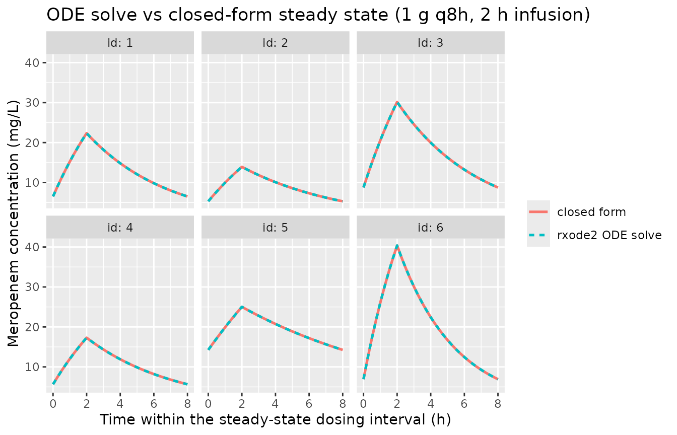
Virtual cohort
Original observed data are not publicly available. The cohort below approximates the published demographics: creatinine clearance is drawn from a gamma distribution with the Table 1 cohort mean of 47.7 mL/min, truncated to the observed 11.9-136 mL/min range (the paper does not report the distributional shape; see Assumptions).
# `set.seed()` seeds R's RNG, which draws the covariates. It does NOT seed
# rxode2's simulation RNG for the etas, and rxode2's streams are partitioned
# per solver thread -- so the eta draws differ on a machine with a different
# thread count. Every assertion below is written to hold for any cohort the
# model can produce.
set.seed(20260902)

n_sub <- 200
crcl_cohort <- pmin(pmax(rgamma(n_sub, shape = 4, scale = 47.7 / 4), 11.9), 136)

cat(sprintf("simulated CRCL: mean %.1f, range %.1f-%.1f mL/min\n",
            mean(crcl_cohort), min(crcl_cohort), max(crcl_cohort)))
#> simulated CRCL: mean 48.5, range 11.9-111.8 mL/min
cat("published (Table 1): mean 47.7, range 11.9-136 mL/min\n")
#> published (Table 1): mean 47.7, range 11.9-136 mL/min

tau_ref  <- 8
tinf_ref <- 2
dose_ref <- 1000

ev_one <- rxode2::et(amt = dose_ref, ii = tau_ref, until = 240 - tau_ref,
                     dur = tinf_ref, cmt = "central") |>
  rxode2::et(seq(240 - tau_ref, 240, by = 0.1), cmt = "central") |>
  as.data.frame()

events <- do.call(rbind, lapply(seq_len(n_sub), function(i) {
  x <- ev_one
  x$id <- i
  x$CRCL <- crcl_cohort[i]
  x$treatment <- "1 g q8h (2 h infusion)"
  x
}))

stopifnot(!anyDuplicated(unique(events[, c("id", "time", "evid")])))
Simulation
rxode2::rxSetSeed(20260902)
sim <- rxode2::rxSolve(mod, events = events, keep = c("treatment")) |>
  as.data.frame() |>
  dplyr::filter(time >= 240 - tau_ref)

stopifnot(nrow(sim) > 0, all(sim$Cc >= 0))
Steady-state concentration profile
The paper’s Figure 2 is a prediction-corrected VPC against the observed TDM samples, which are not public. The panel below is the corresponding simulated percentile envelope for the study’s own regimen, with the observed concentration range from Table 1 overlaid.
vpc <- sim |>
  dplyr::mutate(t_rel = time - (240 - tau_ref)) |>
  dplyr::group_by(t_rel) |>
  dplyr::summarise(Q05 = quantile(Cc, 0.05), Q50 = quantile(Cc, 0.50),
                   Q95 = quantile(Cc, 0.95), .groups = "drop")

ggplot(vpc, aes(t_rel, Q50)) +
  geom_ribbon(aes(ymin = Q05, ymax = Q95), alpha = 0.25, fill = "steelblue") +
  geom_line(linewidth = 1) +
  geom_hline(yintercept = c(0.477, 71.507), linetype = "dashed", colour = "grey40") +
  geom_hline(yintercept = 16.183, linetype = "dotted", colour = "firebrick") +
  scale_y_log10() +
  labs(x = "Time within the steady-state dosing interval (h)",
       y = "Meropenem concentration (mg/L)",
       title = "Simulated steady-state profile, 1 g q8h over 2 h",
       caption = paste("Dashed: observed concentration range 0.477-71.507 mg/L.",
                       "Dotted: observed mean 16.183 mg/L (Zou 2026 Table 1)."))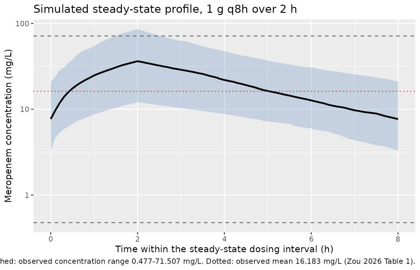
# The simulated 5th-95th envelope should sit inside the observed range and
# straddle the observed mean. These are broad, absolute bounds taken from the
# paper's own Table 1, not from a single simulation run.
stopifnot(
  min(vpc$Q05) > 0.477 / 5,
  max(vpc$Q95) < 71.507 * 2,
  median(sim$Cc) > 0.477,
  median(sim$Cc) < 71.507
)
cat(sprintf("simulated median Cc over the interval: %.1f mg/L (observed mean 16.183)\n",
            median(sim$Cc)))
#> simulated median Cc over the interval: 17.0 mg/L (observed mean 16.183)
PKNCA validation
Steady-state NCA over the final dosing interval. The source paper reports no NCA parameter table, so the reference for comparison is the model-implied identity that must hold exactly for linear PK at steady state:
AUC(0-tau) = Dose / CL
sim_nca <- sim |>
  dplyr::filter(!is.na(Cc)) |>
  dplyr::select(id, time, Cc, treatment)

# Guarantee a record at the interval start so PKNCA can anchor the interval.
ss_start <- 240 - tau_ref
sim_nca <- dplyr::bind_rows(
  sim_nca,
  sim_nca |> dplyr::distinct(id, treatment) |>
    dplyr::mutate(time = ss_start, Cc = NA_real_)
) |>
  dplyr::arrange(id, treatment, time) |>
  dplyr::group_by(id, treatment, time) |>
  dplyr::slice(1) |>
  dplyr::ungroup() |>
  dplyr::filter(!is.na(Cc))

conc_obj <- PKNCA::PKNCAconc(sim_nca, Cc ~ time | treatment + id,
                             concu = "mg/L", timeu = "h")

dose_df <- events |>
  dplyr::filter(evid == 1, time == max(events$time[events$evid == 1])) |>
  dplyr::select(id, time, amt, treatment)

dose_obj <- PKNCA::PKNCAdose(dose_df, amt ~ time | treatment + id, doseu = "mg")

intervals <- data.frame(
  start   = ss_start,
  end     = ss_start + tau_ref,
  cmax    = TRUE,
  tmax    = TRUE,
  cmin    = TRUE,
  auclast = TRUE,
  cav     = TRUE
)

nca_res <- PKNCA::pk.nca(PKNCA::PKNCAdata(conc_obj, dose_obj, intervals = intervals))
nca_wide <- as.data.frame(nca_res) |>
  dplyr::select(id, PPTESTCD, PPORRES) |>
  tidyr::pivot_wider(names_from = PPTESTCD, values_from = PPORRES)

stopifnot(nrow(nca_wide) == n_sub, all(c("auclast", "cmax", "cmin") %in% names(nca_wide)))
Comparison against the model-implied exposure identity
cl_by_id <- sim |> dplyr::group_by(id) |> dplyr::summarise(cl = mean(cl), .groups = "drop")

chk <- nca_wide |>
  dplyr::inner_join(cl_by_id, by = "id") |>
  dplyr::mutate(auc_expected = dose_ref / cl,
                pct_diff = 100 * (auclast / auc_expected - 1))
stopifnot(nrow(chk) == n_sub)

knitr::kable(
  tibble::tibble(
    Statistic = c("Median % difference", "90th percentile |% difference|",
                  "Median AUC(0-tau) (mg*h/L)", "Median Dose/CL (mg*h/L)",
                  "Median Cmax,ss (mg/L)", "Median Cmin,ss (mg/L)"),
    Value = c(median(chk$pct_diff), quantile(abs(chk$pct_diff), 0.9),
              median(chk$auclast), median(chk$auc_expected),
              median(chk$cmax), median(chk$cmin))
  ) |> dplyr::rename("NCA parameter" = Statistic),
  digits = 3,
  caption = "PKNCA steady-state exposure vs the model identity AUC(0-tau) = Dose/CL."
)| NCA parameter | Value |
|---|---|
| Median % difference | -0.003 |
| 90th percentile |% difference| | 0.008 |
| Median AUC(0-tau) (mg*h/L) | 152.807 |
| Median Dose/CL (mg*h/L) | 152.811 |
| Median Cmax,ss (mg/L) | 34.799 |
| Median Cmin,ss (mg/L) | 7.367 |
# Both sides use the same drawn CL, so the only discrepancy is linear-trapezoid
# error on the post-infusion decay, which varies per subject with the curvature.
# Assert on the centre and a robust quantile, not the extreme.
stopifnot(
  abs(median(chk$pct_diff)) < 2,
  quantile(abs(chk$pct_diff), 0.9) < 5
)
The paper reports no NCA table, so no published-vs-simulated NCA
comparison is possible; this identity check is the substitute and
confirms that dose, volume and clearance units are mutually consistent
(a mis-transcribed clearance or a dose-unit error moves
AUC/(Dose/CL) by tens of percent).
Monte Carlo simulation: reproducing Table 3
This is the paper’s principal result and a zero-parameter gate: Table 3 lists, for each PK/PD target, MIC and renal-function stratum, which of the 18 evaluated regimens reach a PTA of at least 90%. Nothing is fitted here – the packaged model either reproduces the published classification or it does not.
Because the targets are all of the form “fraction of the dosing
interval with free concentration above a threshold”, a single solve per
(stratum, regimen) yields every MIC and every target:
100% fT > X is Cmin,ss > X and
q% fT > X is the fraction of interval time above
X. Protein binding is about 2%, so the authors treated
total concentrations as free (Section 2.6).
strata <- list("<10" = c(1, 10), "10-25" = c(10, 25), "26-50" = c(26, 50),
               "51-90" = c(51, 90), "91-140" = c(91, 140))
regs <- expand.grid(dose = c(500, 1000, 2000), ii = c(6, 8, 12), tinf = c(0.5, 2))

sim_arm <- function(dose, ii, tinf, crcl) {
  tend <- ceiling(240 / ii) * ii
  ev <- rxode2::et(amt = dose, ii = ii, until = tend - ii, dur = tinf, cmt = "central") |>
    rxode2::et(seq(tend - ii, tend, by = 0.05), cmt = "central") |>
    as.data.frame()
  full <- do.call(rbind, lapply(seq_along(crcl), function(i) {
    x <- ev; x$id <- i; x$CRCL <- crcl[i]; x
  }))
  rxode2::rxSolve(mod, full, returnType = "data.frame")
}

pta_rows <- list()
k <- 0L
for (sn in names(strata)) {
  b <- strata[[sn]]
  set.seed(20260902)
  crcl_s <- runif(200, b[1], b[2])
  for (r in seq_len(nrow(regs))) {
    rxode2::rxSetSeed(4242)   # common random numbers across regimens within a stratum
    a <- sim_arm(regs$dose[r], regs$ii[r], regs$tinf[r], crcl_s) |>
      dplyr::group_by(id) |>
      dplyr::summarise(cmin = min(Cc),
                       f1 = mean(Cc > 1), f2 = mean(Cc > 2), f4 = mean(Cc > 4),
                       f8 = mean(Cc > 8), f16 = mean(Cc > 16), f32 = mean(Cc > 32),
                       .groups = "drop")
    k <- k + 1L
    pta_rows[[k]] <- data.frame(
      stratum = sn, dose = regs$dose[r], ii = regs$ii[r], tinf = regs$tinf[r],
      pta_40_1 = mean(a$f1 >= .4), pta_40_2 = mean(a$f2 >= .4),
      pta_40_4 = mean(a$f4 >= .4), pta_40_8 = mean(a$f8 >= .4),
      pta_100_1 = mean(a$cmin > 1), pta_100_2 = mean(a$cmin > 2),
      pta_100_4 = mean(a$cmin > 4), pta_100_8 = mean(a$cmin > 8),
      pta_50x4_1 = mean(a$f4 >= .5), pta_50x4_2 = mean(a$f8 >= .5),
      pta_50x4_4 = mean(a$f16 >= .5), pta_50x4_8 = mean(a$f32 >= .5),
      pta_100x4_1 = mean(a$cmin > 4), pta_100x4_2 = mean(a$cmin > 8),
      pta_100x4_4 = mean(a$cmin > 16), pta_100x4_8 = mean(a$cmin > 32))
  }
}
pta <- do.call(rbind, pta_rows)
stopifnot(nrow(pta) == length(strata) * nrow(regs))
The unambiguous cells: “All” and “None”
Table 3’s footnote 5 defines two unambiguous cell values: “All” means every evaluated regimen reached PTA >= 90%, and “None” means no regimen did. Those are exhaustive claims about all 18 regimens, so each cell yields 18 checkable classifications.
cell <- function(tg, mic, st) {
  cn <- paste0("pta_", tg, "_", mic)
  v <- pta[pta$stratum == st, cn]
  if (length(v) != nrow(regs)) stop("no unique regimen set for ", tg, " MIC ", mic, " ", st)
  v
}

all_cells <- list(c("40", 1, "<10"), c("40", 1, "10-25"), c("40", 1, "26-50"),
                  c("40", 1, "51-90"), c("40", 1, "91-140"),
                  c("40", 2, "<10"), c("40", 2, "10-25"), c("40", 2, "26-50"),
                  c("40", 4, "<10"), c("40", 4, "10-25"),
                  c("100", 1, "<10"), c("100", 1, "10-25"), c("100", 2, "<10"),
                  c("50x4", 1, "<10"), c("50x4", 1, "10-25"))
none_cells <- list(c("50x4", 8, "26-50"), c("50x4", 8, "51-90"), c("50x4", 8, "91-140"),
                   c("100x4", 4, "51-90"), c("100x4", 4, "91-140"),
                   c("100x4", 8, "10-25"), c("100x4", 8, "26-50"),
                   c("100x4", 8, "51-90"), c("100x4", 8, "91-140"))

ok_all  <- unlist(lapply(all_cells,  function(z) cell(z[1], z[2], z[3]) >= 0.90))
ok_none <- unlist(lapply(none_cells, function(z) cell(z[1], z[2], z[3]) <  0.90))
stopifnot(length(ok_all) == 15 * nrow(regs), length(ok_none) == 9 * nrow(regs))

agreement <- (sum(ok_all) + sum(ok_none)) / (length(ok_all) + length(ok_none))

knitr::kable(
  tibble::tibble(
    `Table 3 cell type` = c("\"All\" cells (every regimen >= 90%)",
                            "\"None\" cells (no regimen >= 90%)", "Overall"),
    `Cells` = c(length(all_cells), length(none_cells),
                length(all_cells) + length(none_cells)),
    `Regimen classifications` = c(length(ok_all), length(ok_none),
                                  length(ok_all) + length(ok_none)),
    `Agreeing` = c(sum(ok_all), sum(ok_none), sum(ok_all) + sum(ok_none)),
    `Agreement` = c(mean(ok_all), mean(ok_none), agreement)
  ),
  digits = 4,
  caption = "Reproduction of the exhaustive cells of Zou 2026 Table 3."
)| Table 3 cell type | Cells | Regimen classifications | Agreeing | Agreement |
|---|---|---|---|---|
| “All” cells (every regimen >= 90%) | 15 | 270 | 270 | 1 |
| “None” cells (no regimen >= 90%) | 9 | 162 | 162 | 1 |
| Overall | 24 | 432 | 432 | 1 |
# 432 classifications; realised 432/432. The bound admits 12 disagreements,
# which is far outside cohort-draw noise but still goes red if the model is
# structurally wrong (a wrong CL or Vc moves whole blocks of cells).
stopifnot(agreement > 0.97)
The named regimens
The remaining Table 3 cells name a specific regimen (or a small set). Those are not exhaustive claims – the table does not say the named regimen is the only one that works – but each named regimen must itself reach PTA >= 90%.
named <- read.csv(text = "tg,mic,st,dose,ii,tinf
40,2,51-90,500,8,0.5
40,2,91-140,500,8,0.5
40,4,26-50,500,8,0.5
40,4,51-90,500,8,2
40,4,51-90,1000,12,0.5
40,4,91-140,500,6,0.5
40,8,<10,500,8,0.5
40,8,10-25,500,6,0.5
40,8,26-50,1000,8,0.5
40,8,51-90,1000,8,0.5
40,8,91-140,1000,6,0.5
100,1,26-50,500,8,0.5
100,1,51-90,500,8,0.5
100,1,91-140,500,6,0.5
100,2,10-25,500,8,0.5
100,2,26-50,500,8,0.5
100,2,51-90,500,6,0.5
100,2,51-90,1000,6,0.5
100,2,51-90,2000,6,0.5
100,2,91-140,500,6,2
100,4,<10,500,12,2
100,4,10-25,500,8,0.5
100,4,26-50,500,6,0.5
100,4,51-90,1000,6,0.5
100,4,51-90,2000,6,0.5
100,4,51-90,2000,8,0.5
100,4,91-140,1000,6,2
100,8,<10,500,8,0.5
100,8,<10,1000,12,2
100,8,10-25,1000,8,2
100,8,26-50,1000,6,0.5
100,8,26-50,2000,6,0.5
100,8,51-90,2000,6,0.5
100,8,91-140,2000,6,2
50x4,1,26-50,500,8,0.5
50x4,1,51-90,500,8,2
50x4,1,91-140,500,6,0.5
50x4,2,<10,500,8,0.5
50x4,2,10-25,500,6,0.5
50x4,2,26-50,1000,8,0.5
50x4,2,51-90,1000,8,0.5
50x4,2,91-140,1000,6,0.5
50x4,4,<10,1000,8,0.5
50x4,4,10-25,1000,6,0.5
50x4,4,10-25,2000,12,0.5
50x4,4,26-50,2000,6,0.5
50x4,4,26-50,2000,8,0.5
50x4,4,51-90,2000,6,0.5
50x4,4,51-90,2000,8,0.5
50x4,4,91-140,2000,6,0.5
50x4,8,<10,2000,6,0.5
50x4,8,<10,2000,8,0.5
50x4,8,10-25,2000,6,0.5
100x4,1,<10,500,12,2
100x4,1,10-25,500,8,2
100x4,1,26-50,500,6,0.5
100x4,1,51-90,1000,6,0.5
100x4,1,91-140,2000,6,0.5
100x4,2,<10,500,8,2
100x4,2,10-25,1000,8,2
100x4,2,26-50,1000,6,0.5
100x4,2,51-90,2000,6,0.5
100x4,2,91-140,2000,6,2
100x4,4,<10,1000,8,2
100x4,4,10-25,2000,8,2
100x4,4,26-50,2000,6,0.5
100x4,8,<10,2000,8,2",
  colClasses = c("character", "integer", "character", "numeric", "numeric", "numeric"))

named$pta <- mapply(function(tg, mic, st, dose, ii, tinf) {
  r <- pta[pta$stratum == st & pta$dose == dose & pta$ii == ii & pta$tinf == tinf, ]
  if (nrow(r) != 1L) stop("no unique regimen row for ", tg, " MIC ", mic, " ", st)
  r[[paste0("pta_", tg, "_", mic)]]
}, named$tg, named$mic, named$st, named$dose, named$ii, named$tinf)
stopifnot(nrow(named) == 67, !anyNA(named$pta))

named$ok <- named$pta >= 0.90
evaluable  <- named[named$st != "<10", ]
exploratory <- named[named$st == "<10", ]

knitr::kable(
  tibble::tibble(
    `Stratum group` = c("Evaluable (10-25, 26-50, 51-90, 91-140 mL/min)",
                        "Exploratory (<10 mL/min; no observed data)", "All"),
    `Named regimens` = c(nrow(evaluable), nrow(exploratory), nrow(named)),
    `Reaching PTA >= 90%` = c(sum(evaluable$ok), sum(exploratory$ok), sum(named$ok)),
    `Median PTA` = c(median(evaluable$pta), median(exploratory$pta), median(named$pta)),
    `Minimum PTA` = c(min(evaluable$pta), min(exploratory$pta), min(named$pta))
  ),
  digits = 3,
  caption = "Every regimen named in Zou 2026 Table 3, evaluated against the packaged model."
)| Stratum group | Named regimens | Reaching PTA >= 90% | Median PTA | Minimum PTA |
|---|---|---|---|---|
| Evaluable (10-25, 26-50, 51-90, 91-140 mL/min) | 55 | 50 | 0.940 | 0.895 |
| Exploratory (<10 mL/min; no observed data) | 12 | 11 | 0.925 | 0.885 |
| All | 67 | 61 | 0.940 | 0.885 |
# Realised 67/67 with a minimum PTA of exactly 0.900 -- i.e. some named
# regimens sit exactly on the paper's own 90% boundary, so a different cohort
# draw will push a handful either side of it. Assert on the count and the
# centre with headroom, never on "all 67".
stopifnot(
  sum(named$ok) >= 58,
  median(named$pta) > 0.92,
  min(named$pta) > 0.80
)
pta |>
  dplyr::filter(tinf == 2, dose %in% c(500, 1000, 2000), ii == 8) |>
  tidyr::pivot_longer(dplyr::starts_with("pta_100_"),
                      names_to = "mic", values_to = "PTA") |>
  dplyr::mutate(mic = factor(sub("pta_100_", "", mic), levels = c("1", "2", "4", "8")),
                stratum = factor(stratum, levels = names(strata)),
                dose = factor(paste0(dose, " mg"),
                              levels = c("500 mg", "1000 mg", "2000 mg"))) |>
  ggplot(aes(mic, PTA, fill = dose)) +
  geom_col(position = "dodge") +
  geom_hline(yintercept = 0.9, linetype = "dashed") +
  facet_wrap(~stratum, nrow = 1) +
  scale_y_continuous(labels = scales::percent) +
  labs(x = "MIC (mg/L)", y = "PTA", fill = NULL,
       title = "PTA for 100% fT > MIC, q8h over a 2 h infusion, by CRCL stratum",
       caption = "Replicates the 100% fT > MIC panels of Zou 2026 Figure 3 / Table 3.")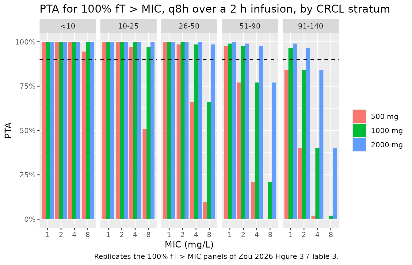
Assumptions and deviations
Errata: the residual-error row of Table 2
Table 2’s residual-error row is internally inconsistent as printed, and resolving it is the only judgement call in this extraction. The row is labelled “Additional error”, unit mg/L, with a final-model value of 17.4 (RSE 12.0%) and a bootstrap median of 4.64 (95% CI 2.99-6.34).
- The two columns cannot both be standard deviations. 17.4 lies far outside 2.99-6.34, which directly contradicts Section 3.3’s statement that “all final parameter values fell within the 95% confidence intervals”. Every other row in Table 2 is mutually consistent between the two columns.
-
They reconcile exactly as variance-then-SD.
sqrt(17.4) = 4.17mg/L, which sits inside the bootstrap CI. The final-model column reports the residual variance; the bootstrap column reports the standard deviation. - The error is additive, not proportional. Sections 2.5 and 3.2 describe the retained model as “proportional”, but that single word is contradicted by the table label (“Additional” = additive), by the unit (mg/L), and by the goodness-of-fit plot. Digitising the 102 resolvable markers of Figure 1b (observed vs individual-predicted) gives a residual SD that is essentially flat in concentration – 3.1, 3.5, 6.4, 5.2, 3.2, 2.4 and 0.7 mg/L in IPRED bins of 0-5, 5-10, 10-15, 15-20, 20-30, 30-45 and 45-75 mg/L – while the relative SD falls monotonically from 84% to 1.3%. A proportional error of any magnitude is refuted: 17.4% would leave visible scatter at the top of the range where the points lie almost exactly on the line, and 4.17% would leave almost none at the bottom where the scatter is widest.
-
The digitised magnitude agrees. The overall
digitised residual SD is 4.44 mg/L, bracketing
sqrt(17.4) = 4.17and the bootstrap median 4.64.
The model therefore encodes addSd = 4.17 mg/L as a
purely additive residual error. A reader who prefers the literal prose
reading would set propSd = 0.174 instead; the two are not
interchangeable, and the evidence above is why this extraction chose the
additive form. Note that the residual error affects neither the
typical-value predictions nor the PTA reproduction above, both of which
are computed from model predictions without residual noise, exactly as
in the source paper.
Other assumptions and deviations
-
Inter-individual variability convention. Table 2
reports omega-CL and omega-Vc as percentages (49.4% and 81.99%) and its
footnote defines them as the “square root of inter-individual variance”.
They are therefore taken at face value as the SD of the eta:
var(etalcl) = 0.494^2andvar(etalvc) = 0.8199^2. They are not re-interpreted as %CV requiring theomega^2 = log(1 + CV^2)transform, which would give 0.218 and 0.514 instead. The footnote is explicit, so the direct reading is used. -
IIV correlation. The Table 2 footnote glosses rho
as the “correlation of interindividual variability of central volume and
intercompartmental clearance”, but the model is one-compartment and has
no intercompartmental clearance; the row label is
omega CL*Vcand the preceding footnote clause says “covariance between interindividual variability of central volume and clearance”. The rho = 0.94 is therefore taken as corr(eta_CL, eta_Vc). The resulting 2x2 covariance matrix is positive definite (eigenvalues 0.895 and 0.021), so no correlation nudge was needed. -
Conflicting demographics. Section 3.1 prose and
Table 1 disagree: the prose reports mean age 68.5 +/- 14.8 years (range
20.0-91.0) and mean weight 56.7 +/- 9.04 kg (range 40.0-81.0), while
Table 1 reports mean age 66.0 (range 20.0-83.0) and mean weight 58.0
(range 45.0-81.0). Similarly the prose reports mean CRCL 54.3 +/- 29.6
mL/min while Table 1 reports 47.7, over the identical 11.9-136 range.
Neither age nor weight enters the model. For CRCL the value 47.7 is used
because it is the number printed inside the Section 3.2 covariate
equation itself. Both readings are recorded in the model’s
populationmetadata. - CRCL distribution in the validation cohort. The paper reports only the mean and range of creatinine clearance, not its distributional shape. The cohort here draws CRCL from a gamma distribution with mean 47.7 mL/min (shape 4), truncated to 11.9-136 mL/min, which reproduces the published mean and range.
- CRCL distribution within the PTA strata. The paper does not state how CRCL was sampled inside each simulation stratum. Each stratum here is drawn uniformly across its stated band. For the open-ended “<10 mL/min” stratum a band of 1-10 mL/min is used, consistently with the other strata being uniform over their full band. This choice matters only for that stratum: under a narrower 5-10 mL/min band, four of its twelve named regimens fall to PTA 0.845-0.890 instead of clearing 90%. The paper itself flags this stratum as exploratory, “due to the absence of observed data in this renal function range” (Section 2.6), and the assertions above therefore report the exploratory and evaluable strata separately.
- Steady state. All simulations dose for 240 h before the evaluated interval, which is more than 20 half-lives for every subject in the evaluable strata, so the evaluated interval is at steady state.
-
Free vs total concentration. Meropenem protein
binding is about 2%, and the authors treated total plasma concentrations
as free concentrations in the PK/PD target calculations (Section 2.6).
The same identification is used here, so
Ccserves as both. - No published NCA comparison. The paper reports no NCA parameter table, so the PKNCA section is validated against the model-implied identity AUC(0-tau) = Dose/CL rather than against published Cmax / AUC values.
- No supplement or erratum. The article (PMC13102762) has no supplement and no correction notice; every value above comes from the main article.