Sirolimus (Wang 2019) • nlmixr2lib

Model and source

Citation: Wang DD, Chen X, Li ZP. Population pharmacokinetics of sirolimus in pediatric patients with kaposiform hemangioendothelioma: A retrospective study. Oncol Lett. 2019;18(3):2412-2419. doi:10.3892/ol.2019.10562
Description: One-compartment population PK model with first-order absorption for oral sirolimus in Chinese children with kaposiform hemangioendothelioma, developed from routine therapeutic-drug-monitoring trough concentrations (Wang 2019). Apparent clearance CL/F rises exponentially with age and alanine aminotransferase and is 0.441-fold lower in girls than in boys; apparent volume V/F rises exponentially with the duration of sirolimus treatment. All covariates enter uncentered. The absorption rate constant is fixed at 0.485 per hour. Inter-individual variability is on CL/F and V/F and the residual error is exponential.
Article: https://doi.org/10.3892/ol.2019.10562 (open access, PMC6676569)

Wang and colleagues fitted a one-compartment model with first-order absorption to 133 routine trough concentrations of oral sirolimus from 17 Chinese children with kaposiform hemangioendothelioma. Age, alanine aminotransferase (ALT) and sex were retained on apparent clearance, and the duration of sirolimus treatment (DTT) on apparent volume. The paper publishes no dose simulation and no NCA table. The validation below therefore uses the paper’s goodness-of-fit and predictive-check figures (Figures 2 and 4), and four other paediatric sirolimus models, to settle two things the paper leaves unstated: the numeric coding of sex, and the scale of the variance parameters.

Population

The cohort is a single-centre retrospective one from the Children’s Hospital of Fudan University, Shanghai, January 2016 to April 2018 (Wang 2019 Table I):

17 patients, 11 male and 6 female.
Age 0.2-6 years (median 0.8) and weight 3.6-18 kg (median 7).
Daily sirolimus dose 0.16-1.5 mg (median 0.5). The starting dose was 0.8 mg/m^2 twice daily, then adjusted by therapeutic drug monitoring to a trough of 10-15 ng/mL.
Treatment duration at sampling 7-749 days (median 117).
ALT 2-120 IU/L (median 21).

Every concentration is a pre-dose trough measured with the Emit 2000 whole-blood assay (LLOQ 3.5 ng/mL, linear to 30 ng/mL). The same information is available programmatically via readModelDb("Wang_2019_sirolimus")()$population.

Source trace

Equation / parameter	Value	Source location
`lcl` (CL/F intercept)	3.19 L/h	Table IV (SE 23.7%); Abstract
`lvc` (V/F at DTT = 0)	165 L	Table IV (SE 26.9%); Abstract
`lka` (Ka)	0.485 1/h, fixed	Table IV; Methods “PPK modeling”
`e_age_cl`	0.215 per year	Table IV (SE 21.7%)
`e_alt_cl`	0.0108 per IU/L	Table IV (SE 18%)
`e_sexf_cl`	-0.818	Table IV (SE 15.4%)
`e_t_firstdose_vc`	0.0783 per 10 days	Table IV (SE 7.8%)
`etalcl`	0.047089 (omega = 0.217, read as SD)	Table IV; Methods equation 1
`etalvc`	1.779556 (omega = 1.334, read as SD)	Table IV; Methods equation 1
`expSd`	0.365	Table IV (SE 6.8%); Methods equation 3
`CL/F = theta * EXP(theta_AGEage) EXP(theta_ALTALT) EXP(theta_SEX*sex)`	n/a	Results “Modeling”, final covariate model
`V/F = theta * EXP[theta_DTT*(DTT/10)]`	n/a	Results “Modeling”, final covariate model
Sex code 1 = male, 2 = female	n/a	Not printed; see “Sex coding” below
DTT in days	n/a	Table I (“Duration of treatment with sirolimus (days)”)
Exponential residual `Y = IPRED * exp(eps)`	n/a	Methods equation 3 (selected by OFV)

mod <- readModelDb("Wang_2019_sirolimus")
ui <- rxode2::rxode(mod)
#> ℹ parameter labels from comments will be replaced by 'label()'
theta <- ui$theta
th <- function(nm) theta[[nm]]

# Typical CL/F with the model's sex code (1 = male, 2 = female). `sex_code`
# lets the literal 0/1 reading be evaluated with the same function.
cl_wang <- function(age, alt, sex_code) {
  exp(th("lcl")) * exp(th("e_age_cl") * age) * exp(th("e_alt_cl") * alt) *
    exp(th("e_sexf_cl") * sex_code)
}
vc_wang <- function(dtt_days) exp(th("lvc")) * exp(th("e_t_firstdose_vc") * dtt_days / 10)

Sex coding

The final clearance equation contains EXP(theta_SEX x sex) with theta_SEX = -0.818, but the paper never states how sex was coded. The direction is not in doubt: the Discussion says “males had a higher CL/F than females of the same age”, so the code increases from male to female, and the female-to-male ratio is exp(-0.818) = 0.441 whatever the coding. Because age and ALT enter uncentered, though, the intercept 3.19 L/h belongs to the subject whose sex code is 0. Under the literal 0/1 reading that subject is a boy. Under a 1/2 coding it is no real subject, and every predicted concentration is 2.27-fold higher than under 0/1. Three independent checks settle it.

Check 1: other paediatric sirolimus models

The table gives typical CL/F for a 7 kg, 0.8-year-old child, the cohort medians. For Wang 2019 it also uses the median ALT of 21 IU/L. The comparator equations are as printed in Fan 2024 Supplementary Table S1 (doi:10.3389/fphar.2024.1457614), which tabulates the paediatric vascular-anomaly sirolimus models, plus the Chen 2021 tuberous-sclerosis model from this library. Chen 2020 comes from the same hospital and disease as Wang 2019, and the two cohorts partly overlap.

wt <- 7
age <- 0.8
pma_wk <- 40 + age * 52.18
external <- tibble::tribble(
  ~model, ~cl,
  "Chen 2020 KHE, CYP3A5\\*3/\\*3", 7.55 * (wt / 70)^0.75,
  "Chen 2020 KHE, CYP3A5\\*1 carrier", 7.55 * (wt / 70)^0.75 * 1.999,
  "Chen 2021 lymphangioma", 11.3 * (wt / 70)^0.75,
  "Chen 2021 tuberous sclerosis", 8.59 * (wt / 70)^0.75,
  "Fan 2024 vascular anomalies", 4.06 * (wt / 16)^1.23,
  "Mizuno 2017 vascular anomalies", 18.5 * (wt / 70)^0.67 * pma_wk^2.94 / (62.9^2.94 + pma_wk^2.94)
)
wang <- tibble::tribble(
  ~model, ~cl,
  "Wang 2019, sex 1/2 (shipped): male", cl_wang(age, 21, 1),
  "Wang 2019, sex 1/2 (shipped): female", cl_wang(age, 21, 2),
  "Wang 2019, literal 0/1: male", cl_wang(age, 21, 0),
  "Wang 2019, literal 0/1: female", cl_wang(age, 21, 1)
)
bind_rows(external, wang) |>
  rename("Model" = model, "CL/F at 7 kg, 0.8 years (L/h)" = cl) |>
  knitr::kable(digits = 2)

Model	CL/F at 7 kg, 0.8 years (L/h)
Chen 2020 KHE, CYP3A53/3	1.34
Chen 2020 KHE, CYP3A5*1 carrier	2.68
Chen 2021 lymphangioma	2.01
Chen 2021 tuberous sclerosis	1.53
Fan 2024 vascular anomalies	1.47
Mizuno 2017 vascular anomalies	2.70
Wang 2019, sex 1/2 (shipped): male	2.10
Wang 2019, sex 1/2 (shipped): female	0.93
Wang 2019, literal 0/1: male	4.75
Wang 2019, literal 0/1: female	2.10


ext_range <- range(external$cl)
ext_gm <- exp(mean(log(external$cl)))
# Cohort (11 male : 6 female) geometric-mean CL/F under each coding.
cohort_gm <- function(male, female) exp((11 * log(male) + 6 * log(female)) / 17)
gm_12 <- cohort_gm(cl_wang(age, 21, 1), cl_wang(age, 21, 2))
gm_01 <- cohort_gm(cl_wang(age, 21, 0), cl_wang(age, 21, 1))
c(external_geomean = ext_gm, wang_sex_1_2 = gm_12, wang_sex_0_1 = gm_01)
#> external_geomean     wang_sex_1_2     wang_sex_0_1 
#>         1.878371         1.571633         3.561262

stopifnot(
  # The 1/2 reading puts the boys (the majority) inside the comparator range...
  cl_wang(age, 21, 1) >= ext_range[1], cl_wang(age, 21, 1) <= ext_range[2],
  # ...and the cohort within 25% of the comparators' geometric mean.
  abs(log(gm_12 / ext_gm)) < log(1.25),
  # The 0/1 reading puts the boys 1.7-fold above the HIGHEST comparator.
  cl_wang(age, 21, 0) / ext_range[2] > 1.6,
  abs(log(gm_01 / ext_gm)) > log(1.8)
)

Under the 1/2 coding the boys sit inside the 1.3-2.7 L/h spread of the five comparator models, and the cohort’s geometric mean is within 25% of theirs. Under the literal 0/1 coding the boys’ 4.75 L/h is 1.8-fold above the highest comparator, and the cohort mean is 1.9-fold above the comparators’. Girls under the 1/2 coding (0.93 L/h) fall below the comparator range. None of the comparators has a sex effect, and the girls are a minority, so this is the expected price of the paper’s large theta_SEX.

Check 2: the level of the population predictions

Figure 2A plots observations against population predictions (PRED) for the final model. The PRED axis runs from about 1 to 37 ng/mL, and the bulk of the points lie between about 5 and 25 ng/mL. Figure 4 is a prediction-corrected VPC. A pcVPC rescales every observation to its bin’s median PRED, so its simulated-median band (the pink band) sits at the cohort’s typical PRED. It lies at about 9-15 ng/mL over the first 7,500 h, where most of the data are. Both figures put the typical population prediction near the paper’s 10-15 ng/mL target.

The virtual cohort below draws age, ALT, daily dose and sampling day from log-normal distributions matched to the Table I medians and means, and truncated to the Table I ranges. It draws sex at 11:6, and gives each child eight trough records, close to the paper’s 133 records over 17 patients.

set.seed(2019)
N_SUBJ <- 200
N_REC <- 8
# Log-normal with the given median and mean, redrawn (not clamped) outside range.
rlnorm_trunc <- function(n, median, mean, lo, hi) {
  s <- sqrt(2 * log(mean / median))
  out <- numeric(0)
  while (length(out) < n) {
    x <- rlnorm(n, log(median), s)
    out <- c(out, x[x >= lo & x <= hi])
  }
  out[seq_len(n)]
}
cohort <- tibble(
  id = seq_len(N_SUBJ),
  SEXF = rbinom(N_SUBJ, 1, 6 / 17),
  AGE = rlnorm_trunc(N_SUBJ, 0.8, 1.21, 0.2, 6),
  ALT = rlnorm_trunc(N_SUBJ, 21, 24.37, 2, 120),
  daily_dose = rlnorm_trunc(N_SUBJ, 0.5, 0.63, 0.16, 1.5)
)
records <- tibble(
  id = rep(cohort$id, each = N_REC),
  day = round(rlnorm_trunc(N_SUBJ * N_REC, 117, 154.2, 7, 749))
)

Each child takes the same twice-daily dose from day 0. A trough is observed just before each morning dose, and T_FIRSTDOSE is updated daily at the same rows, which drives the time-varying V/F.

TAU <- 12
LAST_DAY <- 749
trough_days <- seq_len(LAST_DAY)
events <- bind_rows(lapply(seq_len(N_SUBJ), function(i) {
  obs <- data.frame(
    id = i, time = c(0, trough_days * 24 - 0.01), evid = 0, amt = 0, cmt = "central"
  )
  dose <- data.frame(
    id = i, time = seq(0, LAST_DAY * 24 - TAU, by = TAU), evid = 1,
    amt = cohort$daily_dose[i] / 2, cmt = "depot"
  )
  bind_rows(dose, obs) |>
    arrange(time, desc(evid)) |>
    mutate(
      T_FIRSTDOSE = time, SEXF = cohort$SEXF[i], AGE = cohort$AGE[i], ALT = cohort$ALT[i]
    )
}))

m0 <- rxode2::zeroRe(ui)
solve_troughs <- function(params) {
  # zeroRe() removes the random effects, so rxode2 notes that a multi-subject
  # solve has no omega; any etas are supplied explicitly in `params`.
  s <- suppressWarnings(rxode2::rxSolve(m0, events, params = params, returnType = "data.frame"))
  s[s$time > 0, ] |>
    mutate(day = round((time + 0.01) / 24)) |>
    select(id, day, Cc)
}
zero_eta <- data.frame(etalcl = rep(0, N_SUBJ), etalvc = 0)
pred_12 <- solve_troughs(zero_eta)
# The literal 0/1 coding is the shipped model with the intercept moved by
# -theta_SEX, since (1 + SEXF) and SEXF differ by exactly one code unit.
pred_01 <- solve_troughs(mutate(zero_eta, lcl = th("lcl") - th("e_sexf_cl")))

rec_pred <- records |>
  left_join(rename(pred_12, pred_12 = Cc), by = c("id", "day")) |>
  left_join(rename(pred_01, pred_01 = Cc), by = c("id", "day"))
stopifnot(nrow(rec_pred) == N_SUBJ * N_REC, !anyNA(rec_pred$pred_12), !anyNA(rec_pred$pred_01))

pred_summary <- rec_pred |>
  pivot_longer(c(pred_12, pred_01), names_to = "coding", values_to = "PRED") |>
  mutate(coding = recode(coding, pred_12 = "sex 1/2 (shipped)", pred_01 = "literal 0/1")) |>
  group_by(coding) |>
  summarise(
    `median PRED (ng/mL)` = median(PRED),
    `5th percentile` = quantile(PRED, 0.05),
    `95th percentile` = quantile(PRED, 0.95),
    `% records PRED < 5 ng/mL` = 100 * mean(PRED < 5),
    `% records PRED 5-25 ng/mL` = 100 * mean(PRED >= 5 & PRED <= 25),
    .groups = "drop"
  )
knitr::kable(pred_summary, digits = 1)

coding	median PRED (ng/mL)	5th percentile	95th percentile	% records PRED < 5 ng/mL	% records PRED 5-25 ng/mL
literal 0/1	4.4	1.4	16.2	60.7	38.3
sex 1/2 (shipped)	9.7	3.2	34.6	16.2	73.6


med_12 <- median(rec_pred$pred_12)
med_01 <- median(rec_pred$pred_01)
stopifnot(
  # Figure 4's median band sits at about 9-15 ng/mL and Figure 2A's PRED bulk
  # at 5-25 ng/mL. The two codings differ by a factor of 2.27, far outside any
  # cohort-draw noise (the cohort is drawn with R's RNG and the solve has no
  # random effects, so these values are reproducible).
  med_12 > 7, med_12 < 16,
  med_01 < 6
)

The literal 0/1 coding puts the median population prediction near 4 ng/mL, just above the assay LLOQ and well below both the Figure 4 band and the Figure 2A cloud. The 1/2 coding reproduces them. Figure 4’s x-axis is time since the start of therapy, so the simulated troughs are plotted the same way below, with the virtual records binned at the paper’s bin edges.

bins <- c(0, 700, 1300, 2700, 3600, 5200, 7400, 18000)
rec_pred |>
  mutate(bin = cut(day * 24, bins)) |>
  group_by(bin) |>
  summarise(`sex 1/2 (shipped)` = median(pred_12), `literal 0/1` = median(pred_01), .groups = "drop") |>
  pivot_longer(-bin, names_to = "coding", values_to = "median_pred") |>
  ggplot(aes(bin, median_pred, colour = coding, group = coding)) +
  geom_line() +
  geom_point() +
  annotate("rect", xmin = 0.5, xmax = 6.5, ymin = 9, ymax = 15, alpha = 0.15, fill = "red") +
  labs(
    x = "Time after the start of therapy (h, Figure 4 bins)", y = "Median PRED trough (ng/mL)",
    colour = NULL,
    caption = "Shaded: approximate centre of the Figure 4 simulated-median band over its first six bins."
  ) +
  theme_bw() +
  theme(axis.text.x = element_text(angle = 30, hjust = 1))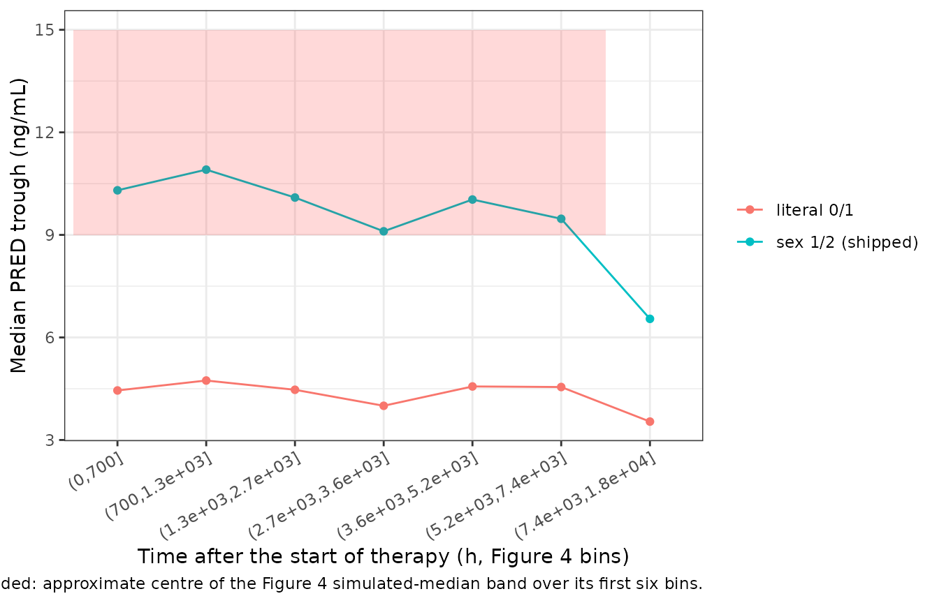

Check 3: the clinical target

The paper states that troughs “were maintained between 10 and 15 ng/ml”. At the cohort medians, the steady-state average concentration for a boy on 0.5 mg/day is 9.9 ng/mL under the 1/2 coding and 4.4 ng/mL under the 0/1 coding. For a TDM cohort titrated to 10-15 ng/mL, only the first is plausible.

c(
  boy_sex_1_2 = 0.5 / 24 / cl_wang(age, 21, 1) * 1000,
  boy_sex_0_1 = 0.5 / 24 / cl_wang(age, 21, 0) * 1000
)
#> boy_sex_1_2 boy_sex_0_1 
#>    9.931717    4.383000

Scale of the variance parameters

Table IV prints omega CL/F = 0.217, omega V/F = 1.334 and sigma 1 = 0.365 without saying whether these are NONMEM variances or their square roots. This group’s other papers, from the Children’s Hospital of Fudan University, print omega as the standard deviation of eta. That has been confirmed against their own simulation figures for several of their tacrolimus and sirolimus models. Wang 2019 has no dose simulation, but its goodness-of-fit plots constrain the residual error directly:

Figure 2B (observations against individual predictions, 133 points). The largest excursions are about 2-fold either way (for example 28 ng/mL at an IPRED of 14, and 7 at 16.5). With a residual SD s on the log scale, the extreme of 133 draws is about 2.6 s.
Figure 2C (|IWRES| against IPRED). The smooth runs at 0.20-0.31, and almost every point is below 1. A sigma-standardised IWRES would have a mean absolute value near 0.8. The axis label is in ng/mL and the magnitudes are about 0.3, so the plotted quantity is the relative residual (DV - IPRED)/IPRED.

# Expected mean |DV/IPRED - 1| and expected largest excursion over 133 records,
# for an exponential residual with log-scale SD s.
mean_abs_rel <- function(s) {
  integrate(function(e) abs(exp(e) - 1) * dnorm(e, 0, s), -10 * s, 10 * s)$value
}
scales <- tibble(
  reading = c("sigma 0.365 is the SD (shipped)", "sigma 0.365 is the variance"),
  s = c(0.365, sqrt(0.365))
) |>
  mutate(
    mean_abs_rel = vapply(s, mean_abs_rel, numeric(1)),
    extreme_fold = exp(qnorm(1 - 0.5 / 133) * s)
  )
scales |>
  rename(
    "Reading" = reading, "Log-scale SD" = s,
    "Expected mean |relative residual|" = mean_abs_rel,
    "Expected extreme fold over 133 records" = extreme_fold
  ) |>
  knitr::kable(digits = 2)

Reading	Log-scale SD	Expected mean \|relative residual\|	Expected extreme fold over 133 records
sigma 0.365 is the SD (shipped)	0.36	0.30	2.65
sigma 0.365 is the variance	0.60	0.55	5.03


stopifnot(
  # Figure 2C smooth 0.20-0.31; Figure 2B extremes about 2-fold. Individual
  # predictions absorb part of the residual (epsilon shrinkage), so the figures
  # should sit somewhat BELOW the expectation, never above it.
  scales$mean_abs_rel[1] > 0.25, scales$mean_abs_rel[1] < 0.35,
  scales$extreme_fold[1] < 3,
  scales$mean_abs_rel[2] > 0.45,
  scales$extreme_fold[2] > 4
)

The SD reading fits both figures with modest shrinkage. The variance reading would put the expected mean relative residual near 0.5 and the extreme near 5-fold, which would take more than 50% epsilon shrinkage to compress into the plotted 2-fold. The omega rows are printed in the same notation in the same table and are read the same way. Figure 2A’s spread about PRED agrees with this: roughly 0.45 on the log scale by eye, against more than 0.8 under the variance reading of all three rows.

Simulation: trough distribution over time

The virtual cohort is simulated with inter-individual variability (etas drawn in R) and the exponential residual, and summarised by Figure 4’s bins after prediction correction. Figure 4 is not reproduced exactly, because the real dosing histories were TDM-titrated and are not available.

etas <- data.frame(
  etalcl = rnorm(N_SUBJ, 0, sqrt(ui$omega["etalcl", "etalcl"])),
  etalvc = rnorm(N_SUBJ, 0, sqrt(ui$omega["etalvc", "etalvc"]))
)
ipred <- solve_troughs(etas)
vpc <- records |>
  left_join(rename(ipred, IPRED = Cc), by = c("id", "day")) |>
  left_join(distinct(select(rec_pred, id, day, PRED = pred_12)), by = c("id", "day")) |>
  mutate(
    DV = IPRED * exp(rnorm(n(), 0, th("expSd"))),
    bin = cut(day * 24, bins)
  ) |>
  group_by(bin) |>
  mutate(pcDV = DV * median(PRED) / PRED) |>
  summarise(
    n = n(),
    p025 = quantile(pcDV, 0.025), p50 = median(pcDV), p975 = quantile(pcDV, 0.975),
    .groups = "drop"
  )
vpc |>
  rename(
    "Bin (h since start)" = bin, "Records" = n, "2.5th (ng/mL)" = p025,
    "Median (ng/mL)" = p50, "97.5th (ng/mL)" = p975
  ) |>
  knitr::kable(digits = 1)

Bin (h since start)	Records	2.5th (ng/mL)	Median (ng/mL)	97.5th (ng/mL)
(0,700]	53	2.1	8.8	23.4
(700,1.3e+03]	200	3.7	9.7	25.5
(1.3e+03,2.7e+03]	507	3.9	9.1	22.8
(2.7e+03,3.6e+03]	272	3.9	8.6	19.9
(3.6e+03,5.2e+03]	266	3.6	9.2	20.4
(5.2e+03,7.4e+03]	172	3.2	8.9	19.6
(7.4e+03,1.8e+04]	130	2.0	6.4	15.1


ggplot(vpc, aes(bin, p50, group = 1)) +
  geom_ribbon(aes(ymin = p025, ymax = p975), alpha = 0.3) +
  geom_line(colour = "red") +
  labs(
    x = "Time after the start of therapy (h, Figure 4 bins)",
    y = "Prediction-corrected trough (ng/mL)",
    caption = "Compare with Figure 4 of Wang 2019 (median band about 9-15 ng/mL)."
  ) +
  theme_bw() +
  theme(axis.text.x = element_text(angle = 30, hjust = 1))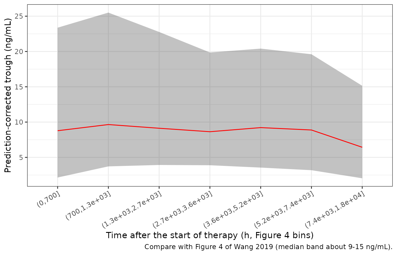


stopifnot(
  # Centre, not extremes: the median of the binned prediction-corrected medians
  # sits in the Figure 4 band region.
  median(vpc$p50) > 6, median(vpc$p50) < 16
)

PKNCA validation

The paper reports no NCA. PKNCA is run after a single 0.25 mg dose in typical children (no random effects) on a sex-by-age grid at the median ALT, with T_FIRSTDOSE held at the median sampling day (117 days, V/F = 412 L) so that disposition is time-invariant. Two identities are checked: AUC0-inf = Dose / CL, and t1/2 = ln 2 * V / CL.

grid <- expand.grid(SEXF = 0:1, AGE = c(0.5, 1, 3)) |>
  mutate(id = row_number(), ALT = 21, T_FIRSTDOSE = 117 * 24)
nca_times <- c(0, seq(0.5, 24, by = 0.5), seq(26, 4000, by = 4))
nca_events <- bind_rows(lapply(grid$id, function(i) {
  rxode2::et(amt = 0.25, cmt = "depot") |>
    rxode2::et(nca_times, cmt = "central") |>
    as.data.frame() |>
    mutate(id = i)
})) |>
  left_join(grid, by = "id")

nca_sim <- rxode2::rxSolve(m0, nca_events, returnType = "data.frame") |>
  select(id, time, Cc) |>
  left_join(select(grid, id, SEXF), by = "id") |>
  mutate(treatment = ifelse(SEXF == 1, "female", "male"))
#> ℹ omega/sigma items treated as zero: 'etalcl', 'etalvc'
#> Warning: multi-subject simulation without without 'omega'

conc <- nca_sim |>
  filter(!is.na(Cc)) |>
  select(id, time, Cc, treatment)
dose <- grid |>
  transmute(id, time = 0, amt = 0.25, treatment = ifelse(SEXF == 1, "female", "male"))

res <- PKNCA::pk.nca(PKNCA::PKNCAdata(
  PKNCA::PKNCAconc(conc, Cc ~ time | treatment + id, concu = "ng/mL", timeu = "h"),
  PKNCA::PKNCAdose(dose, amt ~ time | treatment + id, doseu = "mg"),
  intervals = data.frame(start = 0, end = Inf, cmax = TRUE, tmax = TRUE, aucinf.obs = TRUE, half.life = TRUE)
))
nca <- as.data.frame(res$result)

nca_wide <- nca |>
  filter(PPTESTCD %in% c("cmax", "tmax", "aucinf.obs", "half.life")) |>
  select(id, treatment, PPTESTCD, PPORRES) |>
  pivot_wider(names_from = PPTESTCD, values_from = PPORRES) |>
  left_join(select(grid, id, SEXF, AGE), by = "id") |>
  mutate(
    cl = cl_wang(AGE, 21, 1 + SEXF),
    v = vc_wang(117),
    auc_expected = 0.25 / cl * 1000,
    thalf_expected = log(2) * v / cl
  )

nca_wide |>
  select(treatment, AGE, cmax, tmax, aucinf.obs, auc_expected, half.life, thalf_expected) |>
  rename(
    "Sex" = treatment, "Age (years)" = AGE, "Cmax (ng/mL)" = cmax, "Tmax (h)" = tmax,
    "AUC0-inf (ng*h/mL)" = aucinf.obs, "Dose/CL (ng*h/mL)" = auc_expected,
    "t1/2 (h)" = half.life, "ln2*V/CL (h)" = thalf_expected
  ) |>
  knitr::kable(digits = c(0, 1, 2, 1, 0, 0, 0, 0))

Sex	Age (years)	Cmax (ng/mL)	Tmax (h)	AUC0-inf (ng*h/mL)	Dose/CL (ng*h/mL)	t1/2 (h)	ln2*V/CL (h)
female	0.5	0.59	11.5	288	288	329	329
female	1.0	0.59	11.0	259	259	296	296
female	3.0	0.58	10.0	168	168	192	192
male	0.5	0.58	9.5	127	127	145	145
male	1.0	0.58	9.5	114	114	131	131
male	3.0	0.57	8.5	74	74	85	85


stopifnot(
  nrow(nca_wide) == nrow(grid),
  # Same parameters on both sides; the only differences are the trapezoid and
  # the terminal extrapolation.
  max(abs(nca_wide$aucinf.obs / nca_wide$auc_expected - 1)) < 0.01,
  max(abs(nca_wide$half.life / nca_wide$thalf_expected - 1)) < 0.01
)

Assumptions and deviations

Sex coding (not printed in the paper). Encoded as 1 = male, 2 = female, i.e. exp(-0.818 * (1 + SEXF)). The maintainers asked for an independent verification before choosing between this and the literal 0/1 reading. The three checks above all favour 1/2: five other paediatric sirolimus models, including the same hospital’s Chen 2020 KHE model; the level of the paper’s own population predictions in Figures 2A and 4; and its stated 10-15 ng/mL target. No paper from this group that prints its sex coding was found. Under either coding, girls have 0.441 times the CL/F of boys of the same age and ALT.
Uncentered covariates. Age, ALT and DTT enter uncentered, as printed, so lcl and lvc are equation intercepts (age 0, ALT 0, sex code 0; DTT 0). For the median boy, CL/F is 2.10 L/h.
Scale of omega and sigma. All three Table IV variance rows are read as SDs: omega SDs 0.217 and 1.334 (variances 0.047089 and 1.779556) and residual SD 0.365. This follows the group’s convention and is supported by Figures 2B and 2C (above). The Methods’ boilerplate, “the variance of zero-mean random variables was estimated”, does not say which quantity Table IV prints. This differs from the library’s Wang_2019a_tacrolimus, where a literature comparison table supported the variance reading for that paper.
Duration of treatment and the time-varying V/F. DTT is in days (Table I), supplied as T_FIRSTDOSE in hours and divided by 24 in model(). V/F grows from 175 L at 7 days to 412 L at the median 117 days and about 58,000 L at 749 days. That is not a physiological volume, and it reflects a weakly identified V/F in trough-only data with Ka fixed (bootstrap 95% CI 56-389 L, eta SD 1.334). It is reproduced as published. Because the ODE state is an amount, an increase in V/F at a T_FIRSTDOSE update dilutes the concentration, as it would in NONMEM.
Ka provenance. Ka = 0.485 1/h is printed in Table IV and is what ships. The paper attributes it to its reference 17, Jiao 2009 (Br J Clin Pharmacol), but Jiao_2009_sirolimus in this library fixes Ka at 0.752 1/h.
Residual-error form. Methods equation 3, Y = IPRED * exp(eps), is encoded as lnorm(expSd). The paper does not say whether the data were log-transformed. If they were not, NONMEM’s FOCE-I treats this term as proportional; at an SD of 0.365 the two forms are close.
Figure 4 not reproduced exactly. The individual TDM-titrated dosing histories are not available. The virtual cohort uses constant per-child doses and covariate distributions fitted to the Table I medians, means and ranges.
Covariates without a registered column. MCH, MCHC, and concomitant sulfamethoxazole, digoxin and ursodeoxycholic acid were screened but not retained. They are listed in population$notes rather than covariatesDataExcluded.