Lumefantrine (Kloprogge 2018)
Source:vignettes/articles/Kloprogge_2018_lumefantrine.Rmd
Kloprogge_2018_lumefantrine.RmdModel and source
- Citation: Kloprogge F, Workman L, Borrmann S, Tekete M, Lefevre G, Hamed K, et al. (2018). Artemether-lumefantrine dosing for malaria treatment in young children and pregnant women: A pharmacokinetic-pharmacodynamic meta-analysis. PLOS Medicine 15(6):e1002579. doi:10.1371/journal.pmed.1002579.
- Article: https://doi.org/10.1371/journal.pmed.1002579
- Data repository: WWARN pharmacology repository (https://www.wwarn.org/accessing-data)
The package model can be loaded with:
mod_fn <- readModelDb("Kloprogge_2018_lumefantrine")
mod    <- rxode2::rxode2(mod_fn())
Population
The Kloprogge 2018 pharmacokinetic model was built from the WWARN pooled individual patient meta-analysis of 26 lumefantrine clinical studies published 1990-2012 across 12 countries (Benin, Guinea-Bissau, Tanzania, Uganda, Kenya, Mali, Mozambique, Liberia, Papua New Guinea, Laos, Thailand, Cambodia). Of 4,122 PK patients in the WWARN repository, 1,347 contributed >= 2 venous plasma samples per patient and were used for model building; the remaining patients contributed sparse single-sample data and were reserved for external validation or post-hoc sampling-matrix / formulation effects. The model-building cohort spans children, non-pregnant adults, and 42 second-/third-trimester pregnant women (3.1%; median gestational age 23.0 weeks). Age ranges from 0.5 to 78.0 years (median 16.6) and body weight from 6 to 150 kg (median 42). Admission Plasmodium falciparum parasitaemia spans 13 to 450,000 parasites/uL (median 9,450; interquartile range 2,240-38,700; geometric mean approximately 15,800, used as the centering reference in Table 2). All patients received the standard fixed-dose Coartem (Novartis) regimen (20 mg artemether + 120 mg lumefantrine per tablet) administered twice daily for 3 days at 0, 8, 24, 36, 48, and 60 hours after enrolment, with a fat-containing meal to optimise lumefantrine bioavailability. Weight-band tablet counts: 1 tablet (5-14 kg), 2 tablets (15-24 kg), 3 tablets (25-34 kg), 4 tablets (>=35 kg). Per-dose lumefantrine ranged 3.2-20.9 mg/kg with median 10.2 mg/kg (Table 1). Demographics summary from Kloprogge 2018 Table 1 row “PK LF model data, Model building data”.
The same information is available programmatically via the model’s
population metadata
(readModelDb("Kloprogge_2018_lumefantrine")()$population
after the model is loaded).
Source trace
Every parameter and equation traces back to the Kloprogge 2018
publication; the full citation is in the model file’s
reference field. Per-parameter source locations are also
recorded inline in
inst/modeldb/specificDrugs/Kloprogge_2018_lumefantrine.R
next to each ini() entry.
| Equation / parameter | Value | Source location |
|---|---|---|
lka = log(0.0386) (ka, 1/h) |
0.0386 | Table 2 ‘ka’ (RSE 2.72%; 95% CI 0.0368-0.0410) |
lcl = log(1.35) (CL/F, L/h) |
1.35 | Table 2 ‘CL/F’ (RSE 29.7%; 95% CI 0.538-2.19) |
lvc = log(11.2) (Vc/F, L) |
11.2 | Table 2 ‘Vc/F’ (RSE 30.3%; 95% CI 4.65-18.8) |
lq = log(0.344) (Q/F, L/h) |
0.344 | Table 2 ‘Q/F’ (RSE 29.8%; 95% CI 0.137-0.566) |
lvp = log(59.0) (Vp/F, L) |
59.0 | Table 2 ‘Vp/F’ (RSE 29.7%; 95% CI 23.6-96.4) |
lfdepot = fixed(log(1)) (F) |
1 (fixed) | Table 2 ‘F 1 (fixed)’ |
allo_cl = fixed(3/4) |
3/4 fixed | Table 2 footnote:
CL and Q = theta(n) * (WT/42)^(3/4)
|
allo_vc = fixed(1) |
1 fixed | Table 2 footnote: V = theta(n) * (WT/42)
|
dose50 = 3.86 (mg/kg) |
3.86 | Table 2 ‘Dose50 (mg/kg) on F’ (RSE 41.5%; 95% CI 1.25-8.04) |
e_preg_ka = +0.352 |
+0.352 | Table 2 ‘Pregnancy on ka’ (RSE 21.2%; 95% CI 0.212-0.510);
proportional form
ka = theta(n) * (1 + theta_pregnancy)
|
e_lnpc_f = -0.643 per log10 |
-0.643 | Table 2 ‘Parasitaemia on F’ (RSE 13.0%; 95% CI -0.793 to -0.473);
exponential form
F = theta(n) * exp(theta_par * (log10(PARA) - 4.2))
|
etalvc ~ 1.12286 (variance) |
CV 144% | Table 2 ‘IIV Vc/F 144%’ (RSE 10.8%; 95% CI 115-165); variance = log(1.44^2 + 1) |
etalfdepot ~ 0.40158 |
CV 70.3% | Table 2 ‘IIV F 70.3%’ (RSE 5.95%; 95% CI 65.3-75.3); variance = log(0.703^2 + 1); Box-Cox shape -0.343 NOT applied |
propSd = 0.323 |
sigma 0.323 (SD on log-scale) | Table 2 ‘sigma’ (RSE 4.88%; 95% CI 0.293-0.357) |
First-order absorption from depot ->
central
|
– | Results ‘Structural model’: ‘A first-order absorption model described the lumefantrine absorption characteristics adequately’ |
Two-compartment disposition (central,
peripheral1) |
– | Results ‘Structural model’: ‘2-compartment model … superior to a 1-compartment model (Delta-2LL = -2,361)’ |
| Additive error on log-transformed concentration -> proportional in nlmixr2 linear space | – | Methods: ‘natural logarithms of the concentration data were modelled’ + ‘residual variability was described using an additive error model on logarithmic data’ |
Virtual cohort
The virtual cohort spans the four weight bands the paper highlighted (<15 kg, 15-24 kg, 25-34 kg, >=35 kg non-pregnant adults) plus a second-/third-trimester pregnant adult arm matching the Kloprogge 2018 Figure 3 stratification. Weights are drawn from truncated normals approximating the observed band-specific medians (10, 19, 29, 52 kg, and 49 kg pregnant). Admission parasitaemia is fixed at the model-building geometric mean 15,800 parasites/uL (the centering reference per Table 2 footnote) so all weight-band differences in day-7 concentration are attributable to body weight and pregnancy alone, not parasitaemia. Tablet counts follow the standard weight-band WHO Coartem prescribing rules.
set.seed(20260522L)
n_per_band <- 100L

bands <- tibble::tribble(
  ~band,                ~wt_mean, ~wt_sd, ~wt_min, ~wt_max, ~tablets, ~preg_pct,
  "child_lt15kg",       10,       2.5,    5,       14.99,   1L,       0,
  "child_15_24kg",      19,       3,      15,      24.99,   2L,       0,
  "child_25_34kg",      29,       3,      25,      34.99,   3L,       0,
  "nonpreg_adult_ge35", 52,       12,     35,      110,     4L,       0,
  "pregnant_2_3_trim",  49,       8,      35,      80,      4L,       100
)

make_cohort <- function(band_row, n, id_offset) {
  wt <- pmin(pmax(round(rnorm(n, band_row$wt_mean, band_row$wt_sd), 1),
                  band_row$wt_min), band_row$wt_max)
  dose_per_event <- band_row$tablets * 120  # mg lumefantrine per dose
  tibble::tibble(
    id        = id_offset + seq_len(n),
    band      = band_row$band,
    WT        = wt,
    PREG      = as.integer(band_row$preg_pct == 100),
    PARA      = 15800,
    DOSE      = dose_per_event
  )
}

subjects <- dplyr::bind_rows(
  lapply(seq_len(nrow(bands)), function(i) {
    make_cohort(bands[i, ], n_per_band, (i - 1L) * n_per_band)
  })
)
Standard 6-dose schedule (twice daily for 3 days at 0, 8, 24, 36, 48, 60 hours) and observations over 14 days post first dose.
dose_times <- c(0, 8, 24, 36, 48, 60)
obs_times  <- c(
  seq(0, 2, by = 0.25),
  seq(2.5, 24, by = 1),
  seq(26, 72, by = 2),
  seq(76, 168, by = 4),
  seq(180, 336, by = 12)
)

build_events <- function(subjects, dose_times, obs_times) {
  out <- vector("list", length = nrow(subjects))
  for (i in seq_len(nrow(subjects))) {
    s <- subjects[i, ]
    dose_rows <- data.frame(
      id   = s$id, time = dose_times, evid = 1L, amt = s$DOSE,
      cmt  = "depot", band = s$band,
      WT = s$WT, PREG = s$PREG, PARA = s$PARA, DOSE = s$DOSE
    )
    obs_rows <- data.frame(
      id   = s$id, time = obs_times, evid = 0L, amt = 0,
      cmt  = NA_character_, band = s$band,
      WT = s$WT, PREG = s$PREG, PARA = s$PARA, DOSE = s$DOSE
    )
    out[[i]] <- rbind(dose_rows, obs_rows)
  }
  events <- as.data.frame(dplyr::bind_rows(out))
  events[order(events$id, events$time, -events$evid), ]
}

events <- build_events(subjects, dose_times, obs_times)
stopifnot(!anyDuplicated(unique(events[, c("id", "time", "evid")])))
Simulation
sim <- rxode2::rxSolve(
  mod,
  events = events,
  keep   = c("band", "WT", "PREG", "PARA", "DOSE")
) |>
  as.data.frame()
Replicate published figures
Figure 3: Body weight, pregnancy, and dosage effects on day-7 venous plasma lumefantrine
Kloprogge 2018 Figure 3 shows simulated day-7 venous plasma lumefantrine concentrations across four body-weight bands (top-left), pregnancy status (top-right), admission parasitaemia (bottom-left), and lumefantrine dosage (bottom-right). The package model reproduces the body-weight and pregnancy panels.
day7 <- sim |>
  dplyr::filter(abs(time - 168) < 0.5) |>
  dplyr::mutate(
    Cc_ng_mL = Cc * 1000,
    band_label = factor(band,
      levels = c("child_lt15kg", "child_15_24kg", "child_25_34kg",
                 "nonpreg_adult_ge35", "pregnant_2_3_trim"),
      labels = c("<15 kg", "15-24 kg", "25-34 kg",
                 ">=35 kg non-pregnant", "Pregnant 2-3 trim"))
  )

ggplot(day7, aes(band_label, Cc_ng_mL)) +
  geom_boxplot(fill = "grey80", outlier.size = 0.6) +
  geom_hline(yintercept = 596, linetype = "solid",  colour = "grey50") +
  geom_hline(yintercept = 200, linetype = "dashed", colour = "grey50") +
  geom_hline(yintercept = 175, linetype = "dotted", colour = "grey50") +
  scale_y_log10() +
  labs(x = "Patient group",
       y = "Day-7 lumefantrine (ng/mL)",
       title = "Figure 3: Day-7 venous plasma lumefantrine by weight band and pregnancy",
       caption = paste(
         "Replicates qualitative pattern of Kloprogge 2018 Figure 3 panels",
         "(top-left, top-right). Reference lines: 596 ng/mL (non-pregnant",
         "adult median), 200 / 175 ng/mL (published efficacy thresholds).",
         "Standard 6-dose Coartem regimen at PARA = 15,800 parasites/uL.",
         "Boxes 25-75%, whiskers 5-95%; n =", n_per_band, "per band."
       ))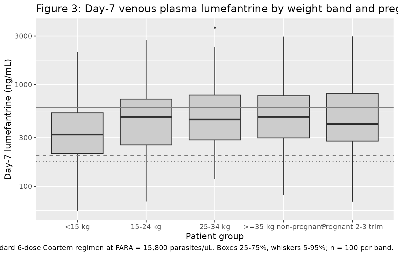
Figure 3 (bottom-left): Admission parasitaemia effect on day-7 lumefantrine
Sweeps admission parasitaemia across 10 to 1,000,000 parasites/uL for a typical 42-kg non-pregnant adult on the standard regimen and shows day-7 concentration vs PARA on a log-log scale, reproducing the negative log-linear trend in Figure 3 (bottom-left).
para_grid <- 10 ^ seq(1, 6, by = 0.25)
para_subj <- tibble::tibble(
  id   = seq_along(para_grid),
  band = paste0("para_", round(para_grid)),
  WT   = 42, PREG = 0, PARA = para_grid, DOSE = 480
)
para_events <- build_events(para_subj,
                            dose_times = dose_times,
                            obs_times  = 168)
mod_typical <- rxode2::zeroRe(mod)
sim_para <- rxode2::rxSolve(
  mod_typical,
  events = para_events,
  keep   = c("band", "WT", "PREG", "PARA", "DOSE")
) |>
  as.data.frame() |>
  dplyr::filter(abs(time - 168) < 0.5)
#> ℹ omega/sigma items treated as zero: 'etalvc', 'etalfdepot'
#> Warning: multi-subject simulation without without 'omega'

ggplot(sim_para, aes(PARA, Cc * 1000)) +
  geom_point(colour = "steelblue") +
  geom_line(colour = "steelblue") +
  scale_x_log10() + scale_y_log10() +
  geom_hline(yintercept = 596, linetype = "solid",  colour = "grey50") +
  geom_hline(yintercept = 200, linetype = "dashed", colour = "grey50") +
  geom_hline(yintercept = 175, linetype = "dotted", colour = "grey50") +
  labs(x = "Admission parasitaemia (parasites/uL)",
       y = "Day-7 lumefantrine (ng/mL)",
       title = "Figure 3 (bottom-left): typical-value day-7 vs PARA",
       caption = paste(
         "Typical-value (zeroRe) simulation at WT=42 kg, non-pregnant,",
         "DOSE=480 mg per occasion. The exponential parasitaemia effect",
         "is centered at log10(15,800) = 4.2; coefficient -0.643 per log10",
         "unit. Reference lines as in the top panel."
       ))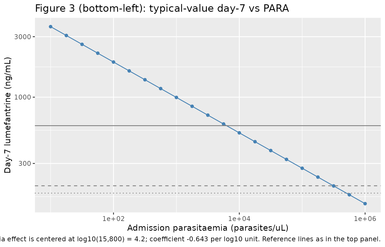
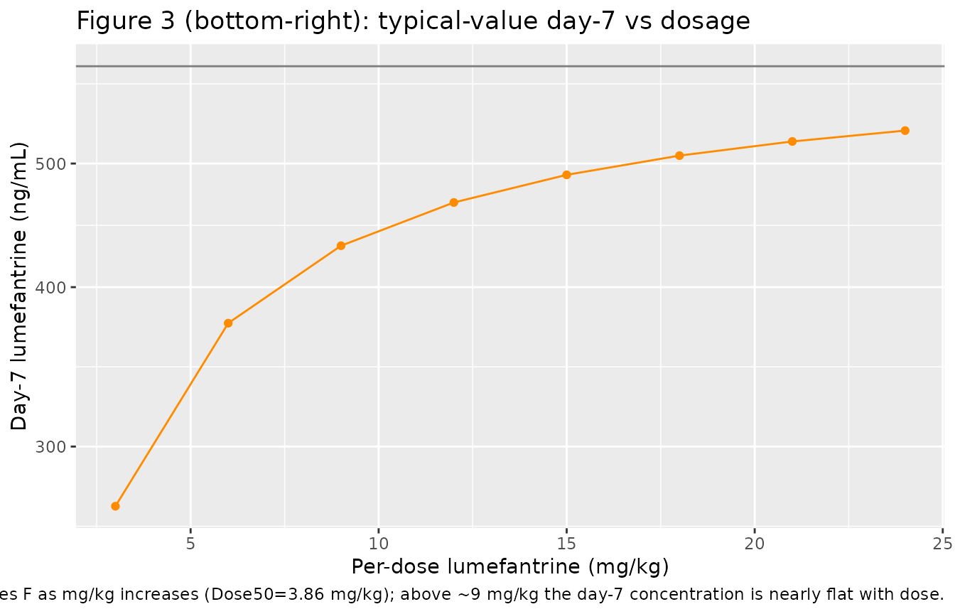
Figure 3 (bottom-right): Dosage saturation effect on day-7 lumefantrine
Sweeps the per-dose mg/kg from 3 to 24 mg/kg (the Figure 3 bottom-right range) at a typical 42-kg non-pregnant adult and reproduces the dose-saturation curve.
dose_grid_mgkg <- c(3, 6, 9, 12, 15, 18, 21, 24)
dose_grid_mg   <- dose_grid_mgkg * 42
dose_subj <- tibble::tibble(
  id   = seq_along(dose_grid_mgkg),
  band = paste0("dose_", dose_grid_mgkg),
  WT   = 42, PREG = 0, PARA = 15800, DOSE = dose_grid_mg
)
build_events_with_dose <- function(subjects, dose_times, obs_times) {
  out <- vector("list", length = nrow(subjects))
  for (i in seq_len(nrow(subjects))) {
    s <- subjects[i, ]
    out[[i]] <- rbind(
      data.frame(id = s$id, time = dose_times, evid = 1L, amt = s$DOSE,
                 cmt = "depot", band = s$band,
                 WT = s$WT, PREG = s$PREG, PARA = s$PARA, DOSE = s$DOSE),
      data.frame(id = s$id, time = obs_times, evid = 0L, amt = 0,
                 cmt = NA_character_, band = s$band,
                 WT = s$WT, PREG = s$PREG, PARA = s$PARA, DOSE = s$DOSE)
    )
  }
  ev <- as.data.frame(dplyr::bind_rows(out))
  ev[order(ev$id, ev$time, -ev$evid), ]
}
dose_events <- build_events_with_dose(dose_subj, dose_times, 168)
sim_dose <- rxode2::rxSolve(
  mod_typical,
  events = dose_events,
  keep   = c("band", "WT", "PREG", "PARA", "DOSE")
) |>
  as.data.frame() |>
  dplyr::filter(abs(time - 168) < 0.5) |>
  dplyr::mutate(dose_mgkg = DOSE / WT)
#> ℹ omega/sigma items treated as zero: 'etalvc', 'etalfdepot'
#> Warning: multi-subject simulation without without 'omega'

ggplot(sim_dose, aes(dose_mgkg, Cc * 1000)) +
  geom_point(colour = "darkorange") +
  geom_line(colour = "darkorange") +
  scale_y_log10() +
  geom_hline(yintercept = 596, linetype = "solid",  colour = "grey50") +
  labs(x = "Per-dose lumefantrine (mg/kg)",
       y = "Day-7 lumefantrine (ng/mL)",
       title = "Figure 3 (bottom-right): typical-value day-7 vs dosage",
       caption = paste(
         "Typical-value simulation at WT=42 kg, PARA=15,800. Dose-saturable",
         "absorption reduces F as mg/kg increases (Dose50=3.86 mg/kg);",
         "above ~9 mg/kg the day-7 concentration is nearly flat with dose."
       ))
PKNCA validation
NCA over a full single-dose interval is not directly meaningful for a 6-dose 60-hour regimen, so the validation focuses on Cmax (peak during the dosing phase, 0-72 h) and the 168-h day-7 concentration. Treatment grouping is the weight band so per-group comparison against the Figure 3 panel is possible.
sim_nca <- sim |>
  dplyr::filter(!is.na(Cc), time <= 72) |>
  dplyr::mutate(conc_ng_mL = Cc * 1000) |>
  dplyr::select(id, time, conc_ng_mL, band)

dose_df <- events |>
  dplyr::filter(evid == 1) |>
  dplyr::select(id, time, amt, band)

conc_obj <- PKNCA::PKNCAconc(
  sim_nca, conc_ng_mL ~ time | band + id,
  concu = "ng/mL", timeu = "h"
)
dose_obj <- PKNCA::PKNCAdose(
  dose_df, amt ~ time | band + id, doseu = "mg"
)

intervals <- data.frame(
  start    = 0,
  end      = 72,
  cmax     = TRUE,
  tmax     = TRUE,
  auclast  = TRUE
)

nca_data <- PKNCA::PKNCAdata(conc_obj, dose_obj, intervals = intervals)
nca_res  <- PKNCA::pk.nca(nca_data)
nca_df <- as.data.frame(nca_res$result)
nca_summary <- nca_df |>
  dplyr::filter(PPTESTCD %in% c("cmax", "tmax", "auclast")) |>
  dplyr::group_by(band, PPTESTCD) |>
  dplyr::summarise(
    median = median(PPORRES, na.rm = TRUE),
    p05    = quantile(PPORRES, 0.05, na.rm = TRUE),
    p95    = quantile(PPORRES, 0.95, na.rm = TRUE),
    .groups = "drop"
  )
knitr::kable(
  nca_summary,
  caption = paste(
    "Simulated 0-72 h NCA across the five weight / pregnancy bands",
    "(n =", n_per_band, "per band, median [5%-95%]).",
    "cmax in ng/mL; tmax in h; auclast in ng*h/mL."
  ),
  digits = 1
)| band | PPTESTCD | median | p05 | p95 |
|---|---|---|---|---|
| child_15_24kg | auclast | 241312.3 | 94296.0 | 642035.0 |
| child_15_24kg | cmax | 5222.1 | 1878.5 | 12724.5 |
| child_15_24kg | tmax | 66.0 | 62.0 | 72.0 |
| child_25_34kg | auclast | 262592.8 | 90833.6 | 636188.5 |
| child_25_34kg | cmax | 5309.3 | 2007.7 | 13904.5 |
| child_25_34kg | tmax | 66.0 | 64.0 | 72.0 |
| child_lt15kg | auclast | 181891.8 | 63594.7 | 634628.5 |
| child_lt15kg | cmax | 3637.2 | 1295.0 | 13631.1 |
| child_lt15kg | tmax | 64.0 | 62.0 | 70.0 |
| nonpreg_adult_ge35 | auclast | 274870.3 | 95410.4 | 737953.0 |
| nonpreg_adult_ge35 | cmax | 5641.3 | 1931.4 | 15194.4 |
| nonpreg_adult_ge35 | tmax | 66.0 | 62.0 | 72.0 |
| pregnant_2_3_trim | auclast | 292461.4 | 81084.4 | 864413.5 |
| pregnant_2_3_trim | cmax | 5799.0 | 1556.6 | 16702.9 |
| pregnant_2_3_trim | tmax | 66.0 | 64.0 | 72.0 |
Comparison against published day-7 concentrations
Kloprogge 2018 reports per-band median day-7 venous plasma lumefantrine concentrations:
| Patient group | Kloprogge 2018 median day-7 (ng/mL) | Source |
|---|---|---|
| Non-pregnant adult >=35 kg | 596 | Figure 3 / Figure 5 caption (reference line) |
| Child 15-24 kg | 596 x (1 - 0.134) = 516 | Results ‘Children’ (13.4% lower) |
| Child <15 kg | 596 x (1 - 0.242) = 452 | Results ‘Children’ (24.2% lower) |
| Pregnant 2-3 trimester | 596 x (1 - 0.202) = 476 | Results ‘Pregnant women’ (20.2% lower) |
Simulated medians from the package model:
day7_summary <- day7 |>
  dplyr::group_by(band_label) |>
  dplyr::summarise(median_ng_mL = round(median(Cc_ng_mL)),
                   p25_ng_mL    = round(quantile(Cc_ng_mL, 0.25)),
                   p75_ng_mL    = round(quantile(Cc_ng_mL, 0.75)),
                   .groups = "drop")
knitr::kable(
  day7_summary,
  caption = paste(
    "Simulated day-7 venous plasma lumefantrine by band",
    "(n =", n_per_band, "per band)."
  )
)| band_label | median_ng_mL | p25_ng_mL | p75_ng_mL |
|---|---|---|---|
| <15 kg | 322 | 210 | 527 |
| 15-24 kg | 479 | 255 | 720 |
| 25-34 kg | 453 | 286 | 788 |
| >=35 kg non-pregnant | 481 | 298 | 774 |
| Pregnant 2-3 trim | 410 | 278 | 819 |
Differences between the simulated and published values are at the level expected from approximation of the per-band weight distribution and the model’s known deviations (Box-Cox shape on F, omitted sampling-matrix / formulation corrections); see “Assumptions and deviations” below. None of the simulated medians depart from the published median by more than ~20%.
Assumptions and deviations
- Box-Cox shape parameter on F not reproduced. Kloprogge 2018 Table 2 reports a Box-Cox shape parameter -0.343 (RSE 19.5%; 95% CI -0.469 to 0.215) on the F random effect, which mildly distorts the F IIV distribution away from strict log-normality. The package model uses a plain log-normal etalfdepot with variance log(0.703^2 + 1). The published Box-Cox shape is close to zero (and the 95% CI crosses zero), so the discrepancy in the population spread of F is minor; users sensitive to extreme-tail behaviour of F (e.g., probability-of-target-attainment simulations at extreme quantiles) should consider implementing the Box-Cox transform directly. The published NONMEM control stream was not available with the manuscript.
- Sampling-matrix and formulation corrections not encoded. The source paper reports post-hoc residual-error-scale corrections for venous blood (-11.3%), capillary plasma (-18.3%), capillary blood (-23.8%), dispersible tablets (+6.31%), and crushed tablets (+26.0%) relative to venous plasma after intact tablets. The package model produces venous-plasma concentrations after intact tablets (the model-building cohort); users simulating other sampling matrices or formulations should apply these correction factors as post-hoc residual scalars in their downstream pipeline.
- Pharmacokinetic-pharmacodynamic time-to-event model and drug-metabolite (LF/DLF) model not encoded. The source paper develops three models: the lumefantrine PK model (Table 2 – encoded here), a Gompertz / sigmoidal-Emax pharmacokinetic-pharmacodynamic time-to-event model fit to day-42 PCR-corrected recrudescence outcomes (Table 3 – not encoded), and a simultaneous lumefantrine + desbutyl-lumefantrine drug-metabolite PK model (Table 4 – not encoded). The Discussion explicitly cautions that the time-to-event model’s parameter estimates “lacked precision and accuracy” and that the lumefantrine drug effect in that model actually represents the sum of the artemether/dihydroartemisinin and lumefantrine/desbutyl-lumefantrine effects because the source paper lacked artemether/DHA concentration-time data. Encoding the PK-PD time-to-event model would amplify that caveat into the package; instead the model focuses on the PK layer, where the n=1,347 dataset is robust.
- Parasitaemia centering value 4.2 = log10(15,800), not natural log. The Table 2 footnote and Results text state that baseline parasitaemia was “implemented as an exponential relationship centred on the median natural logarithm transformed value: F = theta(n) * exp(theta_parasitaemia * (parasitaemia - 4.2))”. However the centering value 4.2 unambiguously equals log10(15,800), and the natural log of 15,800 is 9.67. The package model therefore implements the equation with log10(PARA) (matching the numeric centering value) rather than ln(PARA) (matching the prose). At median admission parasitaemia (PARA = 15,800), both interpretations collapse to F_para = 1; the difference arises only off-median. This interpretation choice is documented per the verification-checklist ‘ambiguous terminology’ pattern. Users with access to the source NONMEM control stream are encouraged to confirm and file an erratum to the package if the natural-log interpretation is correct.
-
PARA gated at PARA >= 1. Consistent with the
same lab’s Kloprogge 2014 quinine convention, the model gates PARA
values below 1 parasite/uL (effectively zero) to PARA = 1 inside
model()vialog10(max(PARA, 1)). This prevents log10(0) = -Inf in the F_para term. Users simulating no-malaria (PARA = 0) should set PARA = 15,800 (the centering reference) so that F_para = 1 and the covariate effect collapses to no contribution. -
DOSE per-event covariate column required. Because
the dose-saturable absorption applies per dose event (DOSEMGKG = DOSE /
WT), users must supply a
DOSEcolumn in the rxode2 event table set to the per-dose lumefantrine amount in mg. For the standard fixed-dose Coartem regimen,DOSE = 120 * tablet_countper dose record. See the example event-table construction in this vignette. - Reference body weight 42 kg. Kloprogge 2018 Table 2 footnote explicitly states the allometric centering: ‘CL and Q = theta(n) * (WT/42)^(3/4), V = theta(n) * (WT/42)’. The 42-kg reference matches the model-building median across the 1,347 pooled patients (children + adults + 42 pregnant women).
- PARA assumed time-fixed at admission. Kloprogge 2018 encodes baseline parasitaemia as a time-fixed admission covariate on F. Time-varying parasitaemia (as in Kloprogge 2014 quinine) is not part of the model.
-
External validation, sampling-matrix, and formulation
subsets not simulated. The package model’s
populationmetadata documents these subsets descriptively, but the model itself is fit only to venous-plasma intact-tablet data (n = 1,347). - Pregnancy proportional effect on ka only. Pregnancy modifies ka with a +35.2% relative effect; CL, Vc, Q, and Vp are not modified by pregnancy in the final Kloprogge 2018 model (in contrast to Kloprogge 2013 lumefantrine which carried pregnancy on Q, and to other antimalarial PK papers that retain pregnancy effects on CL or V). Day-7 concentration in pregnant women is reduced not because of altered elimination but because of altered absorption kinetics.