Wuzhi-capsule lignans as CYP3A4/CYP3A5 inhibitors (He 2021)
Source:vignettes/articles/He_2021_tacrolimus_wuzhi_cyp3a.Rmd
He_2021_tacrolimus_wuzhi_cyp3a.RmdModel and source
- Citation: He Q, Bu F, Zhang H, Wang Q, Tang Z, Yuan J, Lin HS, Xiang X. Investigation of the Impact of CYP3A5 Polymorphism on Drug-Drug Interaction between Tacrolimus and Schisantherin A/Schisandrin A Based on Physiologically-Based Pharmacokinetic Modeling. Pharmaceuticals (Basel). 2021;14(3):198. doi:10.3390/ph14030198. PMCID: PMC7997453. Reversible inhibition constants (Ki): Results 2.1 and Figure 2A,B (STA on CYP3A4 Ki = 0.15 uM, on CYP3A5 Ki = 0.11 uM); Discussion repeats both. Time-dependent inactivation constants: Results 2.2, Discussion, and the Figure 3B annotation (kinact = 0.11 /min, KI = 2.45 uM for CYP3A4); STA produced no TDI on CYP3A5 (Figure 3C). Michaelis-Menten inactivation form kobs = kinact*I/(KI+I) and its estimation by the double-reciprocal plot: Materials and Methods 4.4 and Equation (1). Assay design: Methods 4.3 (RI) and 4.4 (TDI); the underlying data points are in Table S1.
- Article: https://doi.org/10.3390/ph14030198
- PubMed Central open-access copy: https://www.ncbi.nlm.nih.gov/pmc/articles/PMC7997453/
He 2021 co-administer the Wuzhi capsule (a standardised ethanolic extract of Schisandra sphenanthera) with tacrolimus, a combination used in Chinese transplant practice because the extract’s lignans inhibit CYP3A and raise tacrolimus exposure, cutting the required tacrolimus dose. This paper measures, for the two most abundant lignans, schisantherin A (STA) and schisandrin A (SIA), their reversible and time-dependent inhibition of CYP3A4 and CYP3A5 separately, using CYP3A5-genotyped human liver microsomes with CYP3cide to isolate CYP3A5.
This paper contributes two model files, one per lignan:
mod_sta <- rxode2::rxode2(readModelDb("He_2021_schisantherinA_cyp3a"))
mod_sia <- rxode2::rxode2(readModelDb("He_2021_schisandrinA_cyp3a"))

# Fixed and estimated ini() values are not returned as columns by rxSolve(), so
# read them straight off the packaged model when a check needs one.
ini_val <- function(mod, nm) {
  stopifnot(nm %in% mod$iniDf$name)
  mod$iniDf$est[mod$iniDf$name == nm]
}
Scope: what this paper does and does not contribute
He 2021 has two halves, and only one of them is reproducible.
The first half is the authors’ own bench work: reversible-inhibition (RI) and time-dependent-inhibition (TDI) assays that measure the inhibitory potency of STA and SIA on CYP3A4 and CYP3A5, each isoform in its own microsomal system. Every fitted constant is printed, the assay designs are in the Methods, and the underlying data points are in Supplementary Table S1. That is the layer this vignette validates and that the two model files carry.
The second half is a Simcyp V13.1.1 whole-body physiologically based model that integrates those constants (together with the enzyme abundances of Table 4 and the tacrolimus clearance kinetics of Table 3) to predict the fold-increase in tacrolimus AUC in CYP3A5 expressers and non-expressers. That layer is a vendor platform model and is not extracted: the whole-body ODE system is Simcyp’s rather than the authors’, the tissue Kp values were screened and optimised inside the platform, and no project file is deposited. Reconstructing it would require substituting physiology from outside the source. The section “Published results not reproduced here” records what that half produced.
A load-bearing consequence for the in vitro layer: the two isoforms are inhibited by different combinations of the two mechanisms, and each model file records exactly the combination the paper fitted.
| Lignan | Isoform | Reversible (Ki, uM) | Time-dependent (kinact /min, KI uM) |
|---|---|---|---|
| Schisantherin A (STA) | CYP3A4 | 0.15 | 0.11, 2.45 |
| Schisantherin A (STA) | CYP3A5 | 0.11 | none (Figure 3C) |
| Schisandrin A (SIA) | CYP3A4 | little (not fitted) | 0.019, 2.54 |
| Schisandrin A (SIA) | CYP3A5 | 8.74 | 0.014, 2.07 |
In vitro systems
| Assay | CYP3A4 system | CYP3A5 system | Probe | Buffer |
|---|---|---|---|---|
| Reversible inhibition (RI) | CYP3A53/3 HLM, 0.2 mg/mL | CYP3A51/3 HLM + 0.5 uM CYP3cide, 0.2 mg/mL | Tacrolimus disappearance (Dixon plot) | 0.1 M potassium phosphate pH 7.4, 1 mM NADPH, 37 C |
| Time-dependent inhibition (TDI) | CYP3A53/3 HLM, 0.5 mg/mL | CYP3A51/3 HLM + 1.2 uM CYP3cide, 0.5 mg/mL | Testosterone 6-beta-hydroxylation (double-reciprocal plot) | 0.1 M PBS pH 7.4, 1 mM NADPH, 37 C |
CYP3cide (PF-04981517) is a selective mechanism-based inactivator of CYP3A4; it is used to knock out CYP3A4 so that the residual testosterone or tacrolimus turnover in the CYP3A51/3 microsomes is attributable to CYP3A5.
Source trace
Every value in the two model files, with the location it came from.
| Model | Quantity | Value | Source location |
|---|---|---|---|
| He_2021_schisantherinA_cyp3a | ki_3a4 | 0.15 uM | Figure 2A annotation; Results 2.1 |
| He_2021_schisantherinA_cyp3a | ki_3a5 | 0.11 uM | Figure 2B annotation; Results 2.1 |
| He_2021_schisantherinA_cyp3a | ki_inact_3a4 | 2.45 uM | Figure 3B annotation; Discussion |
| He_2021_schisantherinA_cyp3a | kinact_3a4 | 0.11 /min | Figure 3B annotation; Discussion |
| He_2021_schisantherinA_cyp3a | (CYP3A5 TDI) | none | Figure 3C (no inactivation observed) |
| He_2021_schisandrinA_cyp3a | ki_3a5 | 8.74 uM | Figure 2D annotation; Results 2.1 |
| He_2021_schisandrinA_cyp3a | (CYP3A4 RI) | little | Figure 2C (no significant reversible inhibition) |
| He_2021_schisandrinA_cyp3a | ki_inact_3a4 | 2.54 uM | Figure 4B annotation; Discussion |
| He_2021_schisandrinA_cyp3a | kinact_3a4 | 0.019 /min | Figure 4B annotation; Discussion |
| He_2021_schisandrinA_cyp3a | ki_inact_3a5 | 2.07 uM | Figure 4D annotation; Discussion |
| He_2021_schisandrinA_cyp3a | kinact_3a5 | 0.014 /min | Figure 4D annotation; Discussion |
| both | addSd (fixed 0) | 0 | Not reported anywhere; see Assumptions |
| Inactivation-rate form | kobs = kinact*I/(KI+I) | - | Methods 4.4, Equation (1) |
| Inactivation ODE | d/dt(E) = -kobs*E | - | log-linear decay of Figures 3A, 4A, 4C |
| Reversible form | 1/(1 + I/Ki) | - | Competitive inhibition, Dixon plots (Figure 2) |
The eight fitted constants live in the annotations of Figures 2-4 (and are repeated in the Results and Discussion text); they were read from the rendered figure panels, which is why a PDF-to-text pass does not surface all of them. They are the authors’ own reported estimates, not digitised from the plotted points.
Structural identities of the inactivation model
The time-dependent inactivation is a first-order decay whose rate
constant kobs is a hyperbolic (Michaelis-Menten) function
of the inhibitor concentration. These identities are exact by
construction and pin the transcription of kinact and
KI.
kobs <- function(mod, isoform, I) {
  kinact <- ini_val(mod, paste0("kinact_", isoform))
  KI     <- ini_val(mod, paste0("ki_inact_", isoform))
  kinact * I / (KI + I)
}

# 1. kobs(0) = 0 exactly (no inhibitor => no inactivation).
stopifnot(kobs(mod_sta, "3a4", 0) == 0)
stopifnot(kobs(mod_sia, "3a4", 0) == 0)
stopifnot(kobs(mod_sia, "3a5", 0) == 0)

# 2. kobs(KI) = kinact/2 exactly (half-maximal at I = KI).
for (arg in list(list(mod_sta, "3a4"), list(mod_sia, "3a4"), list(mod_sia, "3a5"))) {
  m <- arg[[1]]; iso <- arg[[2]]
  KI <- ini_val(m, paste0("ki_inact_", iso))
  kinact <- ini_val(m, paste0("kinact_", iso))
  stopifnot(abs(kobs(m, iso, KI) - kinact / 2) < 1e-12)
}

# 3. Plateau: kobs approaches kinact at saturating I.
stopifnot(abs(kobs(mod_sta, "3a4", 1e6) - ini_val(mod_sta, "kinact_3a4")) < 1e-6)
Replicating the inactivation time courses (Figures 3A, 4A, 4C)
The ODE d/dt(E) = -kobs * E with E(0) = 1
has the closed-form solution E(t) = exp(-kobs * t), which
is the straight line the authors plot on a log axis. The model is solved
over the assay’s preincubation grid at each measured inhibitor
concentration.
solve_decay <- function(mod, isoform, conc, covname, tmax = 30) {
  ev <- do.call(rbind, lapply(seq_along(conc), function(i) {
    d <- data.frame(id = i, time = seq(0, tmax, by = 1), evid = 0L, cmt = paste0("enzyme_", isoform))
    d[[covname]] <- conc[i]
    d
  }))
  state <- paste0("enzyme_", isoform)
  out <- rxode2::rxSolve(mod, ev, returnType = "data.frame")
  out$conc <- conc[out$id]
  out$activity <- out[[state]]
  out
}

# STA on CYP3A4 (Figure 3A): I = 0, 0.25, 0.5, 1, 2 uM.
sta_3a4 <- solve_decay(mod_sta, "3a4", c(0, 0.25, 0.5, 1, 2), "CP_STA_UM")
#> Warning: multi-subject simulation without without 'omega'

# SIA on CYP3A4 (Figure 4A) and CYP3A5 (Figure 4C): I = 0, 2, 4, 8, 16 uM.
sia_3a4 <- solve_decay(mod_sia, "3a4", c(0, 2, 4, 8, 16), "CP_SIA_UM")
#> Warning: multi-subject simulation without without 'omega'
sia_3a5 <- solve_decay(mod_sia, "3a5", c(0, 2, 4, 8, 16), "CP_SIA_UM")
#> Warning: multi-subject simulation without without 'omega'
# The ODE solution must equal exp(-kobs*t) to solver tolerance.
check_closed_form <- function(df, mod, isoform) {
  df$kobs <- kobs(mod, isoform, df$conc)
  df$analytic <- exp(-df$kobs * df$time)
  max(abs(df$activity - df$analytic))
}
stopifnot(check_closed_form(sta_3a4, mod_sta, "3a4") < 1e-5)
stopifnot(check_closed_form(sia_3a4, mod_sia, "3a4") < 1e-5)
stopifnot(check_closed_form(sia_3a5, mod_sia, "3a5") < 1e-5)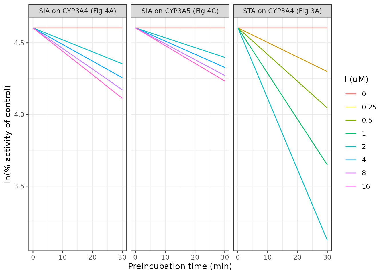
Modelled log-percent CYP activity remaining during preincubation. Replicates the linear-regression lines of He 2021 Figures 3A (STA on CYP3A4), 4A (SIA on CYP3A4) and 4C (SIA on CYP3A5).
Cross-check against the Supplementary Table S1 data points
Table S1 gives the raw natural-log percent-activity readings behind
Figures 3A, 4A and 4C. Regressing each column against preincubation time
recovers an observed kobs per concentration; these must
agree with the model’s kinact*I/(KI+I) prediction. Because
these are experimental means with the authors’ own scatter, the check is
an envelope on the centre and spread of the relative difference, not an
exact bound.
tt <- c(30, 20, 10, 5, 0)
# He 2021 Table S1, Figure 3A (STA on CYP3A4), ln(% activity) at I = 2, 1, 0.5, 0.25 uM.
s1_sta_3a4 <- list(
  I = c(2, 1, 0.5, 0.25),
  m = cbind(
    c(3.0051, 3.1694, 3.5615, 4.0322, 4.6052),
    c(3.5554, 3.8785, 4.0515, 4.1658, 4.5902),
    c(3.9183, 3.9359, 4.0778, 4.2393, 4.6010),
    c(4.2407, 4.2986, 4.3386, 4.4164, 4.6010)
  )
)
# Table S1, Figure 4A (SIA on CYP3A4), I = 16, 8, 4, 2 uM.
s1_sia_3a4 <- list(
  I = c(16, 8, 4, 2),
  m = cbind(
    c(4.0738, 4.2397, 4.3776, 4.4518, 4.6052),
    c(4.1876, 4.2781, 4.3979, 4.5164, 4.6029),
    c(4.2490, 4.3925, 4.4420, 4.5505, 4.6052),
    c(4.3520, 4.4602, 4.5165, 4.5754, 4.6052)
  )
)
# Table S1, Figure 4C (SIA on CYP3A5), I = 16, 8, 4, 2 uM.
s1_sia_3a5 <- list(
  I = c(16, 8, 4, 2),
  m = cbind(
    c(4.1607, 4.2585, 4.3701, 4.4523, 4.5539),
    c(4.2282, 4.4028, 4.4150, 4.4632, 4.6052),
    c(4.2859, 4.4869, 4.5031, 4.4998, 4.6052),
    c(4.3791, 4.4427, 4.5218, 4.5539, 4.6052)
  )
)

observed_kobs <- function(s1) {
  vapply(seq_along(s1$I), function(j) unname(-coef(lm(s1$m[, j] ~ tt))[2]), numeric(1))
}

compare_kobs <- function(s1, mod, isoform) {
  obs <- observed_kobs(s1)
  pred <- kobs(mod, isoform, s1$I)
  100 * (obs - pred) / pred
}

pct_sta_3a4 <- compare_kobs(s1_sta_3a4, mod_sta, "3a4")
pct_sia_3a4 <- compare_kobs(s1_sia_3a4, mod_sia, "3a4")
pct_sia_3a5 <- compare_kobs(s1_sia_3a5, mod_sia, "3a5")

pct_all <- c(pct_sta_3a4, pct_sia_3a4, pct_sia_3a5)
summary(pct_all)
#>    Min. 1st Qu.  Median    Mean 3rd Qu.    Max.
#> -5.1411 -4.1683  0.1875  0.3951  2.8198  9.1075

stopifnot(
  # Centre: a mis-transcribed kinact or KI shifts every column together.
  abs(median(pct_all)) < 10,
  # Envelope: robust to the assay scatter in individual columns.
  quantile(abs(pct_all), 0.9) < 25
)| Panel | I (uM) | Observed kobs (/min) | Model kobs (/min) | Diff (%) |
|---|---|---|---|---|
| STA CYP3A4 (Fig 3A) | 2.00 | 0.0509 | 0.0494 | 3.0 |
| STA CYP3A4 (Fig 3A) | 1.00 | 0.0303 | 0.0319 | -5.0 |
| STA CYP3A4 (Fig 3A) | 0.50 | 0.0203 | 0.0186 | 9.1 |
| STA CYP3A4 (Fig 3A) | 0.25 | 0.0103 | 0.0102 | 1.2 |
| SIA CYP3A4 (Fig 4A) | 16.00 | 0.0167 | 0.0164 | 1.8 |
| SIA CYP3A4 (Fig 4A) | 8.00 | 0.0138 | 0.0144 | -4.0 |
| SIA CYP3A4 (Fig 4A) | 4.00 | 0.0114 | 0.0116 | -1.8 |
| SIA CYP3A4 (Fig 4A) | 2.00 | 0.0083 | 0.0084 | -0.8 |
| SIA CYP3A5 (Fig 4C) | 16.00 | 0.0127 | 0.0124 | 2.8 |
| SIA CYP3A5 (Fig 4C) | 8.00 | 0.0106 | 0.0111 | -5.1 |
| SIA CYP3A5 (Fig 4C) | 4.00 | 0.0088 | 0.0092 | -4.6 |
| SIA CYP3A5 (Fig 4C) | 2.00 | 0.0074 | 0.0069 | 8.3 |
Reversible-inhibition factors
The Dixon-plot inhibition constants enter a victim-drug clearance as
the competitive factor 1/(1 + I/Ki), exposed by each model
as riFactor_*. At I = Ki the factor is exactly
one half, and STA’s much smaller CYP3A5 Ki (0.11 uM) than SIA’s (8.74
uM) makes it the far stronger reversible inhibitor.
ri_factor <- function(I, Ki) 1 / (1 + I / Ki)

# Exact identity at I = Ki.
stopifnot(abs(ri_factor(ini_val(mod_sta, "ki_3a5"), ini_val(mod_sta, "ki_3a5")) - 0.5) < 1e-12)
stopifnot(abs(ri_factor(ini_val(mod_sia, "ki_3a5"), ini_val(mod_sia, "ki_3a5")) - 0.5) < 1e-12)

# STA is the stronger reversible CYP3A5 inhibitor at a common concentration.
I_common <- 0.5
sta_loss <- 1 - ri_factor(I_common, ini_val(mod_sta, "ki_3a5"))
sia_loss <- 1 - ri_factor(I_common, ini_val(mod_sia, "ki_3a5"))
stopifnot(sta_loss > sia_loss)
c(STA_CYP3A5_activity_loss = sta_loss, SIA_CYP3A5_activity_loss = sia_loss)
#> STA_CYP3A5_activity_loss SIA_CYP3A5_activity_loss
#>               0.81967213               0.05411255
Published results not reproduced here
The Simcyp whole-body half predicted the fold-increase (AUC ratio, AUCR) in tacrolimus exposure when co-dosed with each lignan, split by CYP3A5 genotype and by which inhibition mechanism was switched on (Table 2). For a multidose of STA the predicted AUCR was 2.70 in CYP3A5 expressers and 2.41 in non-expressers; SIA raised exposure less. These numbers depend on the enzyme abundances of Table 4, the tacrolimus CYP kinetics of Table 3, the tissue-partition screen and the Simcyp physiology library, none of which is an nlmixr2 ODE model, so they are recorded here rather than reproduced.
Assumptions and deviations
- No residual-error model. The source fits the RI and TDI assays by linear and nonlinear regression and reports only the resulting constants; there is no residual-error model and no assay CV. Per the library convention the additive residual SD is fixed at zero, so each model returns the deterministic published curve.
-
No inter-individual variability. The reported
+/-terms are standard errors of the regression, not between-donor variability, so they are recorded inpopulationand not encoded as an omega. Pooled genotyped microsomes are a single system, not a population. - Constants read from figure annotations. The eight fitted constants are printed in the annotations of Figures 2-4 (and repeated in the Results and Discussion text); they were read from the rendered panels rather than a table. They are the authors’ own estimates.
-
kinact time unit.
kinactis carried in per-minute units, matching the per-minute preincubation-time axis of the assays; the model time unit is minutes. -
No enzyme turnover. The CYP degradation rate
constant
kdeg, which governs the in-vivo magnitude of TDI, is a Simcyp default and is not printed. No turnover term is carried, so the models describe the inactivation phase of the in-vitro assay only; resynthesis is negligible over the 30-minute incubation. - Mechanisms carried per isoform as fitted. STA has no time-dependent inactivation of CYP3A5 (Figure 3C), so that state has no inactivation term; SIA has little reversible inhibition of CYP3A4 (Figure 2C), so that model carries no CYP3A4 reversible constant. Each file records only the mechanism the paper actually fitted for each isoform.
-
In-vivo use requires an unbound driving
concentration. Applying either model to a plasma profile
requires supplying the unbound inhibitor concentration at the site of
enzyme interaction as
CP_STA_UM/CP_SIA_UM; the in-vitro incubation concentration is not a plasma concentration.