Rifampin (Sloan 2017)
Source:vignettes/articles/Sloan_2017_rifampicin.Rmd
Sloan_2017_rifampicin.RmdModel and source
- Citation: Sloan DJ, McCallum AD, Schipani A, Egan D, Mwandumba HC, Ward SA, Waterhouse D, Banda G, Allain TJ, Owen A, Khoo SH, Davies GR. (2017). Genetic determinants of the pharmacokinetic variability of rifampin in Malawian adults with pulmonary tuberculosis. Antimicrob Agents Chemother 61(7):e00210-17. doi:10.1128/AAC.00210-17.
- Description: One-compartment population PK model for oral rifampin in Malawian adults with smear-positive pulmonary tuberculosis (Sloan 2017), developed using a two-stage NONMEM workflow: stage 1 fit a one-compartment + Savic 2007 transit-compartment absorption chain (NN, MTT, Ka) to 47 intensively-sampled patients, then stage 2 fit CL/F and V/F (plus IIVs and a multiplicative sex effect on CL) to 174 sparsely-sampled patients with absorption parameters fixed at the stage 1 estimates; F is fixed at 1, between-subject variability is on CL/F, V/F, and (fixed from stage 1) MTT, and an allometric weight model with fixed exponents 0.75 / 1.0 is referenced to 70 kg.
- Article: Antimicrob Agents Chemother 61(7):e00210-17
Sloan et al. (2017) evaluated whether single-nucleotide polymorphisms in SLCO1B1, AADAC, and CES-1 explained interindividual variability in plasma rifampin exposure among Malawian adults receiving first-line antitubercular therapy. The population PK backbone reported in their Table 3 is a one-compartment model with first-order elimination and a Savic 2007 transit-compartment absorption chain, fit using a two-stage NONMEM workflow: stage 1 fit absorption parameters (Ka, MMT, NN, IIV_MMT) on 47 intensively-sampled patients from a 2007-2008 cohort at Queen Elizabeth Central Hospital, then stage 2 fit disposition parameters (CL/F, V/F, IIV_CL, IIV_V) on 174 sparsely-sampled patients from a 2010-2012 cohort with the stage 1 absorption values held fixed. The only structural covariates retained were allometric weight scaling and a multiplicative sex effect on CL/F; no SNP genotype significantly improved the model fit.
Population
174 adults with smear-positive pulmonary TB were recruited prospectively at Queen Elizabeth Central Hospital in Blantyre, Malawi (2010-2012); all were black Africans. 121 (69.5%) were male; the median age was 30 years (range 17-61), and the median weight was 52 kg (range 34-74). HIV co-infection was present in 98 of 174 (56.3%) – of whom 28 (28.6%) were on antiretroviral therapy at recruitment (median CD4 174 cells/uL, range 6-783). Patients received daily fixed-dose-combination tablets of rifampin and isoniazid per WHO weight-adjusted bands: 300/150 mg (n=2, 1.1%), 450/225 mg (n=113, 64.9%), or 600/300 mg (n=59, 33.9%), corresponding to roughly 8-12 mg/kg rifampin. Sparse PK sampling at predose, 2 h, and 6 h post-dose was performed on day 14 or 21 of TB treatment after an overnight fast (Sloan 2017 Methods ‘Drug plasma concentration determination’).
The 47 intensively-sampled patients that informed the stage 1 absorption parameters were recruited 2007-2008 at the same hospital under similar criteria (Sloan 2017 Methods ‘The intensively sampled pharmacokinetic data’).
The same information is available programmatically via
rxode2::rxode(readModelDb("Sloan_2017_rifampicin"))$population.
Source trace
| Equation / parameter | Value | Source location |
|---|---|---|
| Apparent oral clearance CL/F (female ref, 70 kg) | 19.6 L/h | Sloan 2017 Table 3, row “CL/F (liters/h)” |
| Apparent volume of distribution V/F (70 kg) | 23.6 L | Sloan 2017 Table 3, row “V/F (liters)” |
| Absorption rate constant Ka | 0.277/h (FIX) | Sloan 2017 Table 3, row “Ka (h^-1)” (fixed from stage 1, Table 2) |
| Number of transit compartments NN | 1.5 (FIX) | Sloan 2017 Table 3, row “NN” |
| Mean transit time MMT | 0.326 h (FIX) | Sloan 2017 Table 3, row “MMT (h)” |
| Sex effect on CL (male:female ratio) | 1.2 | Sloan 2017 Table 3, row “THETA_sex_male” |
| Allometric exponent on CL | 0.75 (canonical, fixed) | Sloan 2017 Methods ‘Population pharmacokinetic analysis’ paragraph 4 |
| Allometric exponent on V | 1.0 (canonical, fixed) | Sloan 2017 Methods ‘Population pharmacokinetic analysis’ paragraph 4 |
| Reference body weight | 70 kg | Sloan 2017 Methods ‘Population pharmacokinetic analysis’ paragraph 4 |
| IIV CL (variance, log-normal) | 0.076 | Sloan 2017 Table 3, row “IIVCL” (shrinkage 22%) |
| IIV V (variance, log-normal) | 0.397 | Sloan 2017 Table 3, row “IIVV” (shrinkage 28%) |
| IIV MMT (variance, log-normal) | 0.0706 (FIX) | Sloan 2017 Table 3, row “IIVMMT” (fixed from stage 1) |
| Proportional residual error | 0.22 | Sloan 2017 Table 3, row “Proportional error (%)” |
| Bioavailability F | 1 (fixed) | Sloan 2017 Methods ‘Population pharmacokinetic analysis’ paragraph 4 |
| 1-compartment model + Savic 2007 transit chain | n/a | Sloan 2017 Results paragraph 3 (“a one-compartment model appeared most appropriate with a transit compartment model best describing the absorption phase”) |
Virtual cohort
The original individual-level data are not publicly available. The virtual cohort below matches the published dose distribution (Sloan 2017 Table 1: 300 mg n=2, 450 mg n=113, 600 mg n=59) and demographic summaries. Weights are sampled from a lognormal distribution with median 52 kg and CV 15%, constrained to the published range 34-74 kg; sex is sampled to match the published 30.5% female / 69.5% male fraction (53 of 174 female).
set.seed(20260602)

n_total <- 174L

# Dose distribution from Sloan 2017 Table 1
dose_counts <- tibble::tibble(
  amt_mg = c(300, 450, 600),
  n      = c(2L, 113L, 59L)
)

amt_vec <- rep(dose_counts$amt_mg, dose_counts$n)
amt_vec <- sample(amt_vec)  # shuffle so dose is independent of weight band

# Sample weight: lognormal with median 52, truncated to 34-74 kg.
sample_weight <- function(n, lower = 34, upper = 74, median = 52, cv = 0.15) {
  out <- numeric(0)
  while (length(out) < n) {
    candidates <- stats::rlnorm(
      n,
      meanlog = log(median),
      sdlog   = sqrt(log(1 + cv^2))
    )
    keep <- candidates[candidates >= lower & candidates <= upper]
    out <- c(out, keep)
  }
  out[seq_len(n)]
}
wt_vec <- sample_weight(n_total)

# Sex: 53 female (1), 121 male (0); shuffle independently of dose / weight.
sexf_vec <- sample(rep(c(0L, 1L), c(121L, 53L)))

subj <- tibble::tibble(
  id        = seq_len(n_total),
  amt       = amt_vec,
  WT        = wt_vec,
  SEXF      = sexf_vec,
  treatment = sprintf("%d mg", amt_vec)
)

# Dense sample grid (0.25 h) over 24 h supports VPC and PKNCA terminal-phase
# estimation; the rapid terminal half-life (cl/vc ~ 0.83/h => ~0.84 h) means
# 24 h covers many half-lives.
sample_times <- seq(0, 24, by = 0.25)

dose_rows <- subj |>
  dplyr::transmute(
    id, time = 0, amt, evid = 1L, cmt = "depot",
    WT, SEXF, treatment
  )

obs_rows <- tidyr::expand_grid(id = subj$id, time = sample_times) |>
  dplyr::left_join(
    subj |> dplyr::select(id, WT, SEXF, treatment),
    by = "id"
  ) |>
  dplyr::mutate(amt = 0, evid = 0L, cmt = "central")

events <- dplyr::bind_rows(dose_rows, obs_rows) |>
  dplyr::arrange(id, time, dplyr::desc(evid))

stopifnot(!anyDuplicated(unique(events[, c("id", "time", "evid")])))
Simulation
mod <- rxode2::rxode(readModelDb("Sloan_2017_rifampicin"))
#> ℹ parameter labels from comments will be replaced by 'label()'

set.seed(20260602)
sim <- rxode2::rxSolve(
  mod,
  events = events,
  keep   = c("treatment", "WT", "SEXF")
) |>
  as.data.frame()
Typical-value (no IIV) replication for figure overlays:
mod_typical <- rxode2::zeroRe(mod)
sim_typical <- rxode2::rxSolve(
  mod_typical,
  events = events,
  keep   = c("treatment", "WT", "SEXF")
) |>
  as.data.frame()
#> ℹ omega/sigma items treated as zero: 'etalcl', 'etalvc', 'etalmtt'
#> Warning: multi-subject simulation without without 'omega'
Replicate published figures
Figure 1 - Visual predictive check (VPC)
Sloan 2017 Figure 1 shows a VPC of the final rifampin model with 5th, 50th, and 95th percentile lines overlaid on observed concentration-time data.
sim |>
  dplyr::filter(time > 0) |>
  dplyr::group_by(time) |>
  dplyr::summarise(
    Q05 = stats::quantile(Cc, 0.05, na.rm = TRUE),
    Q50 = stats::quantile(Cc, 0.50, na.rm = TRUE),
    Q95 = stats::quantile(Cc, 0.95, na.rm = TRUE),
    .groups = "drop"
  ) |>
  ggplot(aes(time)) +
  geom_ribbon(aes(ymin = Q05, ymax = Q95), alpha = 0.20) +
  geom_line(aes(y = Q50), linewidth = 0.7) +
  geom_line(aes(y = Q05), linetype = "dashed") +
  geom_line(aes(y = Q95), linetype = "dashed") +
  labs(
    x = "Time post-dose (h)",
    y = "Rifampin Cc (mg/L)",
    title = "Sloan 2017 Figure 1 - VPC of rifampin plasma concentration",
    caption = "Replicates Figure 1 of Sloan 2017 (pooled dose bands; simulated cohort)."
  )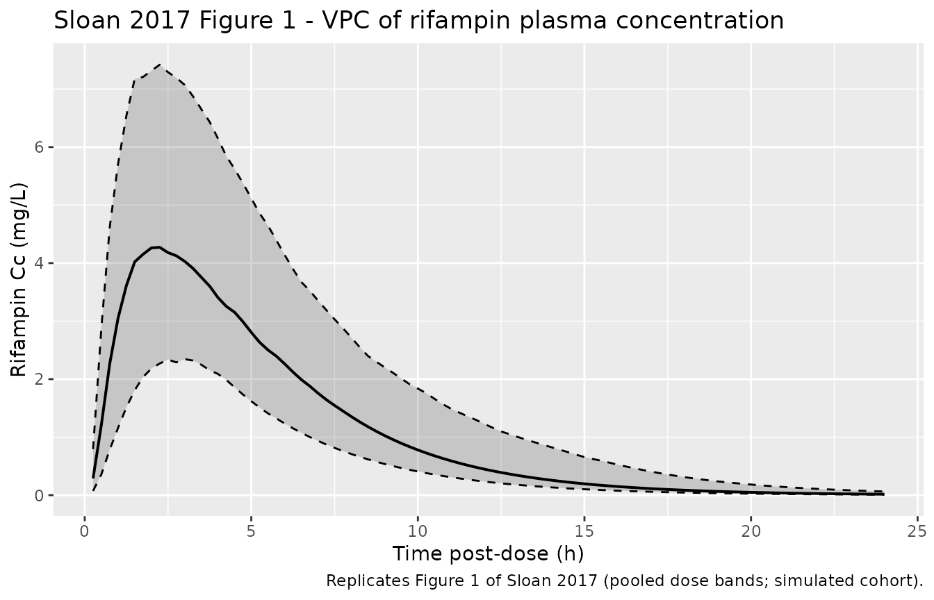
Replicates the structural form of Sloan 2017 Figure 1: VPC of rifampin plasma concentration. Solid line is the simulated median; dashed lines are the 5th and 95th percentiles; shaded ribbon spans the 5th-95th. The simulation pools dose bands as in the paper’s figure.
Cmax distribution by dose band
cmax_per_id <- sim |>
  dplyr::group_by(id, treatment) |>
  dplyr::summarise(
    Cmax = max(Cc, na.rm = TRUE),
    .groups = "drop"
  )

ggplot(cmax_per_id, aes(treatment, Cmax)) +
  geom_boxplot() +
  geom_jitter(width = 0.15, alpha = 0.4, size = 0.7) +
  labs(
    x = "Rifampin dose band",
    y = "Cmax (mg/L)",
    title = "Simulated Cmax by dose band"
  )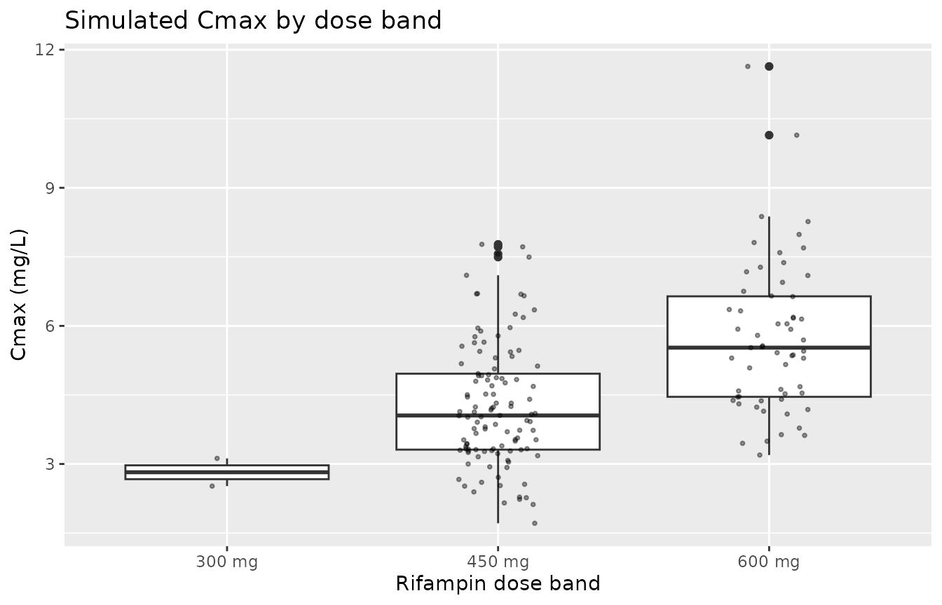
Simulated Cmax distribution stratified by dose band; the rightward shift with dose reflects dose-proportional exposure given F = 1.
PKNCA validation
PKNCA computes Cmax, Tmax, and AUC0-inf grouped by dose band. The
paper reports cohort-level AUC0-inf computed as
dose / (CL/F) using empirical Bayes CL estimates; for the
typical adult on QD dosing the model’s terminal half-life is short
(~0.83 h), so single-dose AUC0-inf is essentially equal to steady-state
AUC0-24.
# Keep the time = 0 pre-dose row (Cc = 0) so PKNCA can anchor AUClast from t = 0;
# omitting it leaves auclast / aucinf.obs NA.
sim_nca <- sim |>
  dplyr::filter(!is.na(Cc)) |>
  dplyr::select(id, time, Cc, treatment) |>
  dplyr::distinct(id, time, .keep_all = TRUE)

dose_df <- events |>
  dplyr::filter(evid == 1) |>
  dplyr::select(id, time, amt, treatment)

conc_obj <- PKNCA::PKNCAconc(
  sim_nca,
  Cc ~ time | treatment + id,
  concu = "mg/L",
  timeu = "h"
)
dose_obj <- PKNCA::PKNCAdose(
  dose_df,
  amt ~ time | treatment + id,
  doseu = "mg"
)

intervals <- data.frame(
  start       = 0,
  end         = Inf,
  cmax        = TRUE,
  tmax        = TRUE,
  aucinf.obs  = TRUE,
  half.life   = TRUE
)

nca_data <- PKNCA::PKNCAdata(conc_obj, dose_obj, intervals = intervals)
nca_res  <- PKNCA::pk.nca(nca_data)
nca_tbl  <- as.data.frame(nca_res$result)
knitr::kable(
  head(nca_tbl, 12),
  caption = "First 12 rows of the per-subject PKNCA result table."
)| treatment | id | start | end | PPTESTCD | PPORRES | exclude | PPORRESU |
|---|---|---|---|---|---|---|---|
| 300 mg | 50 | 0 | Inf | cmax | 2.5194813 | NA | mg/L |
| 300 mg | 50 | 0 | Inf | tmax | 4.5000000 | NA | h |
| 300 mg | 50 | 0 | Inf | tlast | 24.0000000 | NA | h |
| 300 mg | 50 | 0 | Inf | clast.obs | 0.1723095 | NA | mg/L |
| 300 mg | 50 | 0 | Inf | lambda.z | 0.1734984 | NA | 1/h |
| 300 mg | 50 | 0 | Inf | r.squared | 0.9999094 | NA | unitless |
| 300 mg | 50 | 0 | Inf | adj.r.squared | 0.9999057 | NA | unitless |
| 300 mg | 50 | 0 | Inf | lambda.z.time.first | 17.5000000 | NA | h |
| 300 mg | 50 | 0 | Inf | lambda.z.time.last | 24.0000000 | NA | h |
| 300 mg | 50 | 0 | Inf | lambda.z.n.points | 27.0000000 | NA | count |
| 300 mg | 50 | 0 | Inf | clast.pred | 0.1733427 | NA | mg/L |
| 300 mg | 50 | 0 | Inf | half.life | 3.9951224 | NA | h |
Comparison against published NCA
Sloan 2017 Results paragraph 5 reports cohort-level summaries computed from empirical Bayes parameter estimates: median predicted AUC0-inf = 29.9 mg*h/L (range 19.7-63.4); median Cmax = 4.8 mg/L (range 1.4-10.9). The simulated cohort below mixes the published dose-band distribution (300, 450, 600 mg with n = 2, 113, 59) so cohort-level medians are directly comparable.
nca_summary <- nca_tbl |>
  dplyr::filter(PPTESTCD %in% c("cmax", "aucinf.obs")) |>
  dplyr::group_by(PPTESTCD) |>
  dplyr::summarise(
    median = stats::median(PPORRES, na.rm = TRUE),
    minv   = min(PPORRES, na.rm = TRUE),
    maxv   = max(PPORRES, na.rm = TRUE),
    .groups = "drop"
  )

published <- tibble::tibble(
  PPTESTCD        = c("cmax", "aucinf.obs"),
  endpoint        = c("Cmax (mg/L)", "AUC0-inf (mg*h/L)"),
  observed_median = c(4.8, 29.9),
  observed_range  = c("1.4-10.9", "19.7-63.4")
)

compare <- nca_summary |>
  dplyr::left_join(published, by = "PPTESTCD") |>
  dplyr::transmute(
    endpoint,
    simulated_median = round(median, 2),
    simulated_range  = sprintf("%.2f - %.2f", minv, maxv),
    observed_median,
    observed_range
  )

knitr::kable(
  compare,
  caption = "Simulated vs Sloan 2017 published cohort-level rifampin NCA medians."
)| endpoint | simulated_median | simulated_range | observed_median | observed_range |
|---|---|---|---|---|
| AUC0-inf (mg*h/L) | 28.31 | 10.36 - 74.04 | 29.9 | 19.7-63.4 |
| Cmax (mg/L) | 4.46 | 1.71 - 11.64 | 4.8 | 1.4-10.9 |
Assumptions and deviations
Empirical weight distribution. The original individual weight data are not published; the virtual cohort samples WT from a truncated lognormal with median 52 kg and CV 15%, constrained to the published range 34-74 kg. The cohort-level medians are insensitive to this within reasonable shapes.
Empirical sex assignment. Sex was assigned by random shuffle so that the 30.5% female fraction matches the paper without being correlated to dose band. The paper does not break out sex distribution by dose band, so this independence assumption is conservative.
Sex-on-CL table-vs-prose discrepancy. Sloan 2017 Table 3 reports THETA_sex_male = 1.2 (95% CI 1.0-1.3); the Results paragraph 4 describes “an increase of clearance of 17% in male patients.” A 17% increase corresponds to a ratio of 1.17, not 1.20; the model follows the table’s rounded value of 1.2 per the convention of preferring the source’s primary parameter table over its narrative description. The 95% CI 1.0-1.3 is consistent with either interpretation.
Dose assignment. Doses are assigned by sampling each subject from the published n=2/113/59 distribution without conditioning on weight band. The actual trial used WHO weight-band guidelines (8-12 mg/kg) so dose was correlated with weight; the AUC distribution is similar under either assignment because allometric scaling uses the same exponent for CL across the cohort.
Pharmacogenetic SNPs. The packaged model does not encode any of the five SNPs Sloan 2017 screened (SLCO1B1 rs11045819, rs4149032; AADAC rs1803155, rs61733692; CES-1 rs12149368) because none significantly improved the model fit (Sloan 2017 Results paragraph 7). They are documented in the model’s
covariatesDataExcludedmetadata for users who wish to explore them in sensitivity analyses.Steady-state vs single-dose. Sloan 2017 sampled blood on day 14 or 21 at steady state; the model’s short terminal half-life (~0.83 h) makes accumulation under QD dosing negligible, so single-dose AUC0-inf is essentially equal to steady-state AUC0-24. The vignette simulates a single dose for simplicity; users interested in multi-dose steady-state simulations can rerun rxSolve with the standard rxode2 multi-dose event-table idiom.
Errata. A search for published corrections to Sloan et al. 2017 Antimicrob Agents Chemother 61(7):e00210-17 returned no erratum or corrigendum at the time of extraction (2026-06-02).