Amodiaquine seasonal malaria chemoprevention (Ding 2020)
Source:vignettes/articles/Ding_2020_amodiaquine.Rmd
Ding_2020_amodiaquine.RmdModel and source
- Citation: Ding J, Coldiron ME, Assao B, Guindo O, Blessborn D, Winterberg M, Grais RF, Koscalova A, Langendorf C, Tarning J (2020). Adherence and population pharmacokinetic properties of amodiaquine when used for seasonal malaria chemoprevention in African children. Clinical Pharmacology & Therapeutics 107(5):1179-1188.
- Article: https://doi.org/10.1002/cpt.1707 (open access, PMC7232861).
- The final NONMEM control stream is printed at the end of the paper’s
Supplementary Material S1 (“NONMEM code for final population PK model”).
It is the primary source for the model structure and for every
ini()value; the values agree with Table 1 of the main paper.
mod <- rxode2::rxode2(readModelDb("Ding_2020_amodiaquine")())
mod_typ <- rxode2::zeroRe(mod)
Population
The PK cohort was a convenience sample of 136 children aged 3-59 months (78/136, 57.4%, male) from households near the Epicentre study centre in Magaria District, Niger. They received a directly observed course of seasonal malaria chemoprevention (SMC) in November 2016, about 4.5 weeks after the fourth monthly SMC round: a single dose of sulfadoxine-pyrimethamine with the first of three once-daily amodiaquine doses (57.5 mg for ages 3-11 months, 153 mg for ages 12-59 months). Each child gave capillary blood (dried on filter paper) in 3 of 6 pre-defined windows between 0 h and 35 days after the first dose, 404 samples in total. Body weight was not measured; it was predicted from age with a regression derived from 127,256 rural Nigerien children (Supplementary Material S1, equations 2-4), and the predicted median weight (10 kg) is the allometric reference. The four preceding SMC rounds were assumed fully taken and included in the fit.
Source trace
| Item | Value | Source |
|---|---|---|
| Structure: first-order absorption, 2-cmt AQ, 3-cmt DEAQ, 100% molar conversion | ADVAN5, 6 compartments | S1 $MODEL/$PK; S1 Methods “Population PK
analysis”; Figure 1 |
lka |
2.85 1/h | Table 1; S1 THETA(3) |
lcl |
101 L/h | Table 1; S1 THETA(1) |
lvc |
314 L | Table 1; S1 THETA(2) |
lq |
119 L/h | Table 1; S1 THETA(5) |
lvp |
1,820 L | Table 1; S1 THETA(6) |
lfdepot |
1 (held constant) | Table 1; S1 THETA(4) |
lcl_deaq |
2.33 L/h | Table 1; S1 THETA(7) |
lvc_deaq |
49.1 L | Table 1; S1 THETA(8) |
lq_deaq |
2.31 L/h | Table 1 (S1 THETA(9) prints 2.3) |
lvp_deaq |
363 L | Table 1; S1 THETA(10) |
lq2_deaq |
4.34 L/h | Table 1; S1 THETA(11) |
lvp2_deaq |
98.1 L | Table 1; S1 THETA(12) |
lpna50 |
4.66 months | Table 1; S1 THETA(13) |
lpna50_deaq |
2.42 months | Table 1; S1 THETA(14) |
e_wt_cl, e_wt_vc
|
0.75, 1 | S1 equations 5-6; $PK (WT/10)**0.75,
(WT/10)
|
Maturation PNA / (pna50 + PNA)
|
on CL AQ and CL DEAQ | S1 equation 7; Table 1 footnote |
etalcl, etalvc, etalka,
etalfdepot
|
0.0493, 0.646, 3.0, 0.141 | S1 $OMEGA 1-4; Table 1 CV 22.2, 80.4, 173, 37.5% |
etalcl_deaq, etalvp_deaq
|
0.0232, 0.466 | S1 $OMEGA 7 and 10; Table 1 CV 15.2, 68.3% |
expSd, expSd_deaq
|
0.829, 0.204 | Table 1 sigma; S1 $SIGMA 0.688, 0.0417 (variances) |
| Output units nmol/L |
S2 = V2/1000 with AMT in umol |
S1 $INPUT, $PK
|
| Weight from age | WT = 5.46 + 0.162 * age (months) | S1 equation 4 |
Virtual cohort
The paper gives the age range (3-59 months) and median (36 months) of the PK cohort but not its distribution, so ages are drawn uniformly over whole months 3-59. Weight is then predicted from age with the paper’s own pooled regression (Supplementary Material S1, equation 4), exactly as in the analysis, and the dose follows the age band.
set.seed(2020)
rxode2::rxSetSeed(2020)
n_sub <- 200
cohort <- data.frame(id = seq_len(n_sub), PNA = sample(3:59, n_sub, replace = TRUE)) |>
  mutate(
    WT = 5.46 + 0.162 * PNA,
    dose = ifelse(PNA < 12, 57.5, 153),
    treatment = ifelse(PNA < 12, "57.5 mg (3-11 months)", "153 mg (12-59 months)")
  )
count(cohort, treatment)
#>               treatment   n
#> 1 153 mg (12-59 months) 170
#> 2 57.5 mg (3-11 months)  30

obs_times <- sort(unique(c(seq(0, 72, by = 1), seq(78, 168, by = 6), seq(192, 24 * 84, by = 24))))
make_events <- function(subj, dose_times = c(0, 24, 48)) {
  doses <- tidyr::crossing(subj, time = dose_times) |>
    mutate(amt = dose, evid = 1L, cmt = "depot", dvid = NA_integer_)
  obs <- tidyr::crossing(subj, time = obs_times) |>
    mutate(amt = NA_real_, evid = 0L, cmt = NA_character_, dvid = 1L)
  bind_rows(doses, obs) |> arrange(id, time, desc(evid))
}
events <- make_events(cohort)
Simulation
Observation rows carry dvid = 1 with no
cmt; rxode2 returns both observables (Cc for
amodiaquine, Cc_deaq for desethylamodiaquine) as columns on
every row.
Replicate published figures
Concentration-time profiles (cf. Figure 2)
Figure 2 of the paper is a VPC against the observed data, which are not available; the simulated 5th, 50th and 95th percentiles for the 12-59 month dose band (153 mg daily) are shown on the same log axes. Amodiaquine is shown only to 300 h, the window the paper modelled for amodiaquine.
pi_df <- sim |>
  filter(treatment == "153 mg (12-59 months)", time > 0) |>
  select(id, time, Amodiaquine = Cc, Desethylamodiaquine = Cc_deaq) |>
  pivot_longer(c(Amodiaquine, Desethylamodiaquine), names_to = "analyte", values_to = "conc") |>
  filter(analyte == "Desethylamodiaquine" | time <= 300) |>
  group_by(analyte, time) |>
  summarise(p05 = quantile(conc, 0.05), p50 = median(conc), p95 = quantile(conc, 0.95),
            .groups = "drop")
ggplot(pi_df, aes(time / 24, p50)) +
  geom_ribbon(aes(ymin = p05, ymax = p95), alpha = 0.25) +
  geom_line() +
  scale_y_log10() +
  facet_wrap(~analyte, scales = "free") +
  labs(x = "Time after first dose (days)", y = "Concentration (nmol/L)")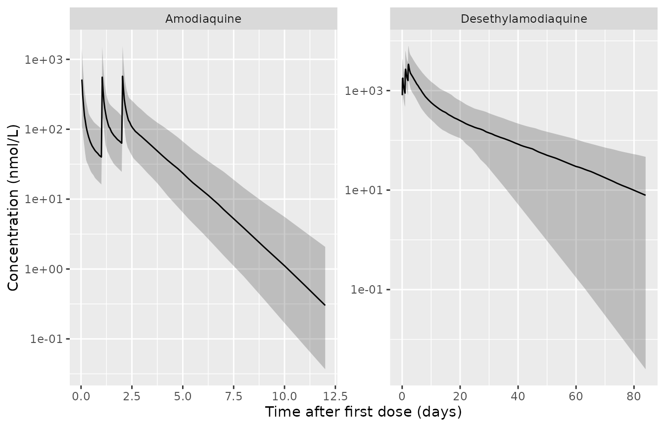
Simulated 5th, 50th and 95th percentiles (153 mg daily for 3 days, ages 12-59 months); compare with Figure 2 of Ding 2020.
Exposure versus age (cf. Figure S1a)
Figure S1a shows total desethylamodiaquine exposure after 10
mg/kg/day for 3 days by age, with the equation-4 weight assigned to each
age. For a typical child with complete conversion, total DEAQ exposure
is exactly the molar dose divided by CL_DEAQ, so the
typical-value curve can be drawn in closed form from the model’s own
clearance.
ages <- data.frame(id = 1:57, PNA = 3:59) |> mutate(WT = 5.46 + 0.162 * PNA, dose = 10 * WT)
ev_age <- ages |>
  tidyr::crossing(time = c(0, 24, 48)) |>
  mutate(amt = dose, evid = 1L, cmt = "depot", dvid = NA_integer_) |>
  bind_rows(mutate(ages, time = 72, amt = NA_real_, evid = 0L, cmt = NA_character_, dvid = 1L)) |>
  arrange(id, time, desc(evid))
typ_age <- rxode2::rxSolve(mod_typ, ev_age, keep = c("PNA", "WT"), returnType = "data.frame") |>
  filter(time == 72) |>
  mutate(auc_deaq = 3 * 10 * WT / 355.85 * 1e6 / cl_deaq) # mmol * 1e6 / (L/h) = h*nmol/L
#> ℹ omega/sigma items treated as zero: 'etalcl', 'etalvc', 'etalka', 'etalfdepot', 'etalcl_deaq', 'etalvp_deaq'
#> Warning: multi-subject simulation without without 'omega'
ggplot(typ_age, aes(PNA, auc_deaq / 1000)) +
  geom_line() +
  labs(x = "Age (months)", y = "DEAQ AUC0-inf (h x umol/L)")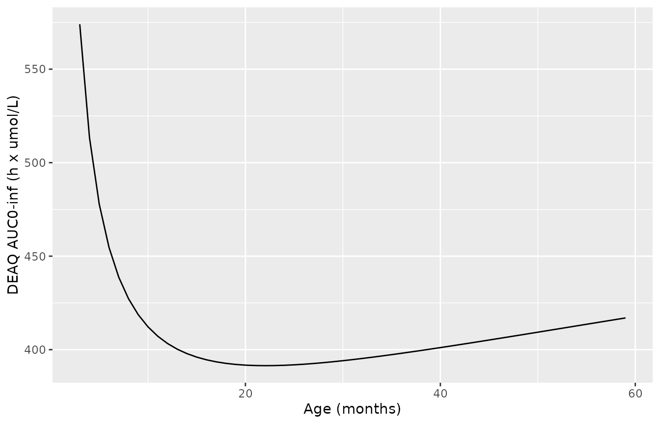
Typical desethylamodiaquine AUC0-inf after 10 mg/kg/day for 3 days by age; compare with Figure S1a of Ding 2020.
Exposure is highest in the youngest children because maturation lowers clearance faster than weight-based dosing lowers the dose, the pattern the paper describes.
PKNCA validation
NCA is run on the individual predictions over the whole 3-day course (a single interval from the first dose to infinity), which is how the paper’s Table 1 secondary parameters were derived (from the empirical Bayes estimates, without residual error).
nca_in <- sim |>
  select(id, time, treatment, Amodiaquine = Cc, Desethylamodiaquine = Cc_deaq) |>
  pivot_longer(c(Amodiaquine, Desethylamodiaquine), names_to = "analyte", values_to = "conc") |>
  filter(!is.na(conc)) |>
  filter(analyte == "Desethylamodiaquine" | time <= 300)
conc_obj <- PKNCA::PKNCAconc(nca_in, conc ~ time | treatment + analyte + id)
intervals <- data.frame(start = 0, end = Inf, cmax = TRUE, tmax = TRUE, aucinf.obs = TRUE,
                        half.life = TRUE)
nca_res <- PKNCA::pk.nca(PKNCA::PKNCAdata(conc_obj, intervals = intervals))
#> No dose information provided, calculations requiring dose will return NA.
nca_tab <- as.data.frame(nca_res)
summary(nca_res)
#>  start end             treatment             analyte   N        cmax
#>      0 Inf 153 mg (12-59 months)         Amodiaquine 170  560 [71.2]
#>      0 Inf 153 mg (12-59 months) Desethylamodiaquine 170 3540 [47.7]
#>      0 Inf 57.5 mg (3-11 months)         Amodiaquine  30  384 [79.1]
#>      0 Inf 57.5 mg (3-11 months) Desethylamodiaquine  30 1850 [46.1]
#>               tmax   half.life    aucinf.obs
#>  49.0 [49.0, 54.0] 28.0 [4.90]  12500 [55.4]
#>  52.0 [49.0, 69.0]   323 [177] 557000 [48.7]
#>  49.0 [49.0, 61.0] 35.8 [6.93]  13200 [57.3]
#>   52.0 [49.0, 102]   343 [184] 440000 [49.2]
#>
#> Caption: cmax, aucinf.obs: geometric mean and geometric coefficient of variation; tmax: median and range; half.life: arithmetic mean and standard deviation; N: number of subjects
Closed-form mass-balance gate
With complete molar conversion, each subject’s desethylamodiaquine
AUC0-inf equals F * total molar dose / CL_DEAQ exactly. The
NCA value differs only by trapezoidal and extrapolation error.
par_ind <- sim |>
  group_by(id) |>
  slice(1) |>
  ungroup() |>
  select(id, cl_deaq, fdepot) |>
  left_join(cohort, by = "id")
chk <- nca_tab |>
  filter(analyte == "Desethylamodiaquine", PPTESTCD == "aucinf.obs") |>
  mutate(id = as.integer(as.character(id))) |>
  left_join(par_ind, by = "id") |>
  mutate(auc_exact = fdepot * 3 * dose / 355.85 * 1e6 / cl_deaq,
         pct_diff = 100 * (PPORRES - auc_exact) / auc_exact)
summary(chk$pct_diff)
#>       Min.    1st Qu.     Median       Mean    3rd Qu.       Max.
#> -0.4409140 -0.0339426 -0.0003491 -0.0207921  0.0150891  0.0341453
stopifnot(
  abs(median(chk$pct_diff)) < 2,
  quantile(abs(chk$pct_diff), 0.9) < 5
)
Comparison against published secondary parameters
Table 1 reports medians over the empirical Bayes estimates of the 136 children (AUC in h x umol/L, converted here to h x nmol/L). The terminal half-lives are compared as NCA values.
ref <- data.frame(
  analyte = c("Amodiaquine", "Desethylamodiaquine"),
  cmax = c(835, 3272),
  aucinf.obs = c(14.76e3, 576e3),
  half.life = c(27.1, 11.0 * 24)
)
sim_cmp <- nca_tab |>
  filter(PPTESTCD %in% c("cmax", "aucinf.obs", "half.life")) |>
  select(analyte, PPTESTCD, PPORRES)
cmp <- nlmixr2lib::ncaComparisonTable(
  simulated = sim_cmp,
  reference = ref,
  by = "analyte",
  units = c(cmax = "nmol/L", aucinf.obs = "h*nmol/L", half.life = "h"),
  tolerance_pct = 20
)
knitr::kable(cmp, digits = 1, caption = paste(
  "Simulated cohort median versus Ding 2020 Table 1 (median of empirical Bayes estimates).",
  attr(cmp, "footnote")
))| NCA parameter | analyte | Reference | Simulated | % diff |
|---|---|---|---|---|
| Cmax (nmol/L) | Amodiaquine | 835 | 530 | -36.5%* |
| Cmax (nmol/L) | Desethylamodiaquine | 3270 | 3310 | +1.2% |
| AUC0-∞ (obs) (h*nmol/L) | Amodiaquine | 14800 | 12600 | -14.9% |
| AUC0-∞ (obs) (h*nmol/L) | Desethylamodiaquine | 576000 | 531000 | -7.8% |
| t½ (h) | Amodiaquine | 27.1 | 28.1 | +3.7% |
| t½ (h) | Desethylamodiaquine | 264 | 291 | +10.1% |
Desethylamodiaquine Cmax, both AUCs and both half-lives agree with Table 1 within 20%. Amodiaquine Cmax is flagged: the simulated cohort median is about a third below the published median. That published value is a median of empirical Bayes estimates, and the absorption rate constant carries a 173% CV with 42.8% shrinkage (Table 1), so the individual estimates are pulled toward the typical absorption rate while a stochastic simulation draws the full spread of slow absorbers, which blunts the amodiaquine peak. Desethylamodiaquine, formed slowly, is insensitive to this. The typical child (36 months, 153 mg daily, random effects set to zero) reproduces the published amodiaquine Cmax closely:
ev_typ <- make_events(data.frame(id = 1, PNA = 36, WT = 5.46 + 0.162 * 36, dose = 153,
                                 treatment = "typical"))
sim_typ <- rxode2::rxSolve(mod_typ, ev_typ, returnType = "data.frame")
#> ℹ omega/sigma items treated as zero: 'etalcl', 'etalvc', 'etalka', 'etalfdepot', 'etalcl_deaq', 'etalvp_deaq'
c(Cmax_AQ = max(sim_typ$Cc), Cmax_DEAQ = max(sim_typ$Cc_deaq))
#>   Cmax_AQ Cmax_DEAQ
#>  794.3682 3633.5761
Adherence methodology (Table 3 and Results)
The paper simulated a typical child (36 months, 11.5 kg, 153 mg daily) under the 4 (first-dose DOT) and 8 (non-DOT) dosing scenarios of Table 3, took the desethylamodiaquine concentration at a given percentile of the fully adherent scenario as the cut-off, and reported the sensitivity (the fraction of simulated non-adherent children falling below it). The cut-off percentiles are the Youden-optimal values the paper reports. Residual error is added to the individual predictions because the method is applied to measured concentrations; scenario 8 (no dose) is assigned zero. The paper used 2,000 children per scenario; 200 are used here. With only 200 fully adherent children the cut-off quantile itself is noisy (it moves the sensitivity by several percentage points), so the scenarios share common random numbers: the same 200 children (the same random effects, reseeded before each scenario’s solve, and the same residual draws) are simulated under every dosing pattern, and only the doses differ.
scen <- list(S1 = c(1, 1, 1), S2 = c(1, 1, 0), S3 = c(1, 0, 1), S4 = c(1, 0, 0),
             S5 = c(0, 1, 1), S6 = c(0, 1, 0), S7 = c(0, 0, 1), S8 = c(0, 0, 0))
n_arm <- 200
days <- c(3, 7, 14, 21, 28)
eps_adh <- rnorm(n_arm * length(days), 0, 0.204)
solve_scenario <- function(dose_t) {
  obs <- expand.grid(id = seq_len(n_arm), time = 24 * days) |>
    mutate(amt = NA_real_, evid = 0L, cmt = NA_character_, dvid = 1L)
  dos <- expand.grid(id = seq_len(n_arm), time = dose_t) |>
    mutate(amt = 153, evid = 1L, cmt = "depot", dvid = NA_integer_)
  ev <- bind_rows(dos, obs) |>
    mutate(PNA = 36, WT = 11.5) |>
    arrange(id, time, desc(evid))
  rxode2::rxSetSeed(2021)
  s <- rxode2::rxSolve(mod, ev, returnType = "data.frame") |> arrange(id, time)
  s$obs <- s$Cc_deaq * exp(eps_adh)
  s
}
sim_adh <- bind_rows(lapply(names(scen)[1:7], function(k) {
  mutate(solve_scenario(c(0, 24, 48)[scen[[k]] == 1]), scenario = k)
}))
# Scenario 8 (no dose taken) has no drug: every concentration is zero.
sim_adh <- bind_rows(sim_adh, filter(sim_adh, scenario == "S1") |>
  mutate(scenario = "S8", Cc_deaq = 0, obs = 0))

sensitivity <- function(pct, day, nonadherent) {
  x <- sim_adh[sim_adh$time == 24 * day, ]
  cutoff <- quantile(x$obs[x$scenario == "S1"], pct / 100)
  100 * mean(x$obs[x$scenario %in% nonadherent] < cutoff)
}
dot <- c("S2", "S3", "S4")
nondot <- c("S2", "S3", "S4", "S5", "S6", "S7", "S8")
adh <- data.frame(
  regimen = rep(c("First-dose DOT", "Non-DOT"), each = 4),
  day = rep(c(3, 7, 14, 28), 2),
  cutoff_pct = c(20, 20, 25, 30, 20, 20, 20, 25),
  paper_sens = c(71, 65, 66, 68, 77, 73, 71, 72)
)
adh$sim_sens <- mapply(function(p, d, r) sensitivity(p, d, if (r == "Non-DOT") nondot else dot),
                       adh$cutoff_pct, adh$day, adh$regimen)
adh |>
  dplyr::rename("Regimen" = regimen, "Day" = day, "Cut-off percentile" = cutoff_pct,
                "Paper sensitivity (%)" = paper_sens, "Simulated sensitivity (%)" = sim_sens) |>
knitr::kable(digits = 0, caption = "Sensitivity at the optimal cut-off percentiles (Ding 2020 Results).")| Regimen | Day | Cut-off percentile | Paper sensitivity (%) | Simulated sensitivity (%) |
|---|---|---|---|---|
| First-dose DOT | 3 | 20 | 71 | 74 |
| First-dose DOT | 7 | 20 | 65 | 68 |
| First-dose DOT | 14 | 25 | 66 | 68 |
| First-dose DOT | 28 | 30 | 68 | 67 |
| Non-DOT | 3 | 20 | 77 | 80 |
| Non-DOT | 7 | 20 | 73 | 76 |
| Non-DOT | 14 | 20 | 71 | 73 |
| Non-DOT | 28 | 25 | 72 | 72 |
stopifnot(
  abs(median(adh$sim_sens - adh$paper_sens)) < 5,
  all(abs(adh$sim_sens - adh$paper_sens) < 10)
)
At the conservative 5th-percentile cut-off the paper reports sensitivities of 22-45% (DOT) and 35-55% (non-DOT):
p5 <- sapply(days, function(d) c(DOT = sensitivity(5, d, dot), nonDOT = sensitivity(5, d, nondot)))
colnames(p5) <- paste("Day", days)
knitr::kable(p5, digits = 0, caption = "Simulated sensitivity (%) at the 5th-percentile cut-off.")| Day 3 | Day 7 | Day 14 | Day 21 | Day 28 | |
|---|---|---|---|---|---|
| DOT | 53 | 44 | 36 | 34 | 19 |
| nonDOT | 62 | 55 | 49 | 48 | 34 |
The simulated ranges span the published ones, running a few points wider at both ends: sensitivity is highest shortly after dosing and falls as the desethylamodiaquine profiles of the scenarios converge.
The paper’s dose-timing sensitivity analysis compared the day-28 5th-percentile cut-off after all three doses on day 1 with full adherence and found a relative difference below 23% (about 10 nmol/L):
sim_t <- solve_scenario(c(0, 0, 0))
p5_same_day <- quantile(sim_t$obs[sim_t$time == 672], 0.05)
p5_full <- quantile(sim_adh$obs[sim_adh$scenario == "S1" & sim_adh$time == 672], 0.05)
c(full_adherence = unname(p5_full), all_on_day1 = unname(p5_same_day),
  relative_diff_pct = unname(100 * (p5_same_day - p5_full) / p5_full))
#>    full_adherence       all_on_day1 relative_diff_pct
#>          36.34889          31.76777         -12.60319
Taking all three doses on day 1 lowers the day-28 cut-off by a relative difference (printed above) inside the paper’s bound of 23%.
Assumptions and deviations
-
Typographical slips in the printed control stream.
The Supplementary Material S1
$PKblock has three evident slips, corrected here: (i) the maturation factors are defined asMF_AQ/MF_DEAQbut applied asMF1/MF2; (ii)F1 = TVF1 * EXP(ETA4)is read asEXP(ETA(4));-
Q1 = TVQ1 * EXP(ETA(3))would give the amodiaquine inter-compartmental clearance the absorption-rate random effect. It is read asEXP(ETA(5)), which is held at zero, because every other parameter uses its own sequential eta index,OMEGA(5)is the zero-valued “AQ IIV inter-compartment clearance” entry, and Table 1 reports no IIV on Q/F AQ. So Q/F AQ carries no IIV in this model.
-
-
Omega values. The S1
$OMEGAand$SIGMAblocks are headed “Initial estimates” but are the final estimates: the square root of each value reproduces the Table 1 “CV for IIV” and sigma entries to the printed precision. (Table 1’s footnote gives the CV assqrt(exp(omega) - 1), but its numbers aresqrt(omega); the variances themselves are used here.) - Q1/F DEAQ. Table 1 prints 2.31 L/h and the control stream 2.3; the Table 1 value is used.
- Molar conversion. The paper fitted molar amounts (dose in umol). The model takes doses in mg of amodiaquine base and applies the base molecular weights (355.85 and 327.81 g/mol, as in the library’s other amodiaquine models) to form the metabolite and report nmol/L; this is numerically identical to the paper’s molar system.
-
Weight is a predicted covariate. The paper never
measured weight; users reproducing the analysis should derive
WTfrom age with equation 4 (WT = 5.46 + 0.162 * PNA), as done in this article. Measured weights can be supplied instead, but that is an extrapolation of the model. - Specimen. Concentrations are capillary whole blood dried on filter paper, not plasma.
- Age distribution. Only the range and median of the PK cohort are reported; a uniform age distribution over 3-59 months is assumed for the virtual cohort, which puts its median age (and hence exposure) somewhat below the paper’s cohort.
- Adherence day definition. “Day 3” etc. is taken as 72 h etc. after the first dose; the typical child of the adherence analysis uses the paper’s stated 11.5 kg rather than the equation-4 weight at 36 months (11.3 kg).
- Previous SMC rounds. The fit assumed the four previous monthly rounds were taken; the simulations here start from a drug-free state, which omits a small residual desethylamodiaquine carry-over.
-
Not retained covariates. Weight-for-age Z-score on
bioavailability and sex were tested but not retained; they are
documented in the model’s
covariatesDataExcludedmetadata.