Bictegravir drug-drug interactions with CYP3A and UGT1A1 perpetrators (Stader 2021)
Source:vignettes/articles/Stader_2021_bictegravir_ddi_pbpk.Rmd
Stader_2021_bictegravir_ddi_pbpk.RmdModel and source
- Citation: Stader F, Battegay M, Marzolini C. Physiologically-Based Pharmacokinetic Modeling to Support the Clinical Management of Drug-Drug Interactions With Bictegravir. Clin Pharmacol Ther. 2021;110(5):1231-1239. doi:10.1002/cpt.2221. Model code: Supplementary Material s002 (CPT_Matlab_Code, the Matlab source of the PBPK framework with the drug library Drug/DrugLibrary/*.m); voriconazole and cobicistat inputs: Supplementary Table S1. The bictegravir drug model is described in Stader F et al. Clin Pharmacol Ther. 2021;109(4):1025-1029, doi:10.1002/cpt.2178.
- Description: PBPK (whole-body, Stader et al. Matlab 2017a framework, as deposited with the paper). Drug-drug interactions of oral bictegravir with inhibitors and inducers of CYP3A and UGT1A1 in adults aged 20 to 50 years. Three drugs are carried simultaneously, each with the framework’s full 63-state whole-body model (16 organs with vascular, interstitial and intracellular sub-compartments, venous and arterial blood, and a compartmental absorption and transit gut) plus 12 enzyme-turnover states (hepatic CYP3A4, 2C19, 2D6, 2C8, 1A2, 2A6, 2B6, 2J2 and UGT1A1, intestinal CYP3A4 per segment): 225 ODEs. The victim drug (bictegravir) takes the bare state names; the two co-administered drugs are parameterised slots (_perpetrator, _perpetrator2) that ship set to voriconazole and rifampicin, and the drugLibrary metadata holds the as-run inputs of all 13 drug models of the deposited library so that any of the paper’s scenarios can be reproduced by substituting them. Interactions act on enzyme synthesis (induction), degradation (mechanism-based inactivation) and turnover rate (competitive inhibition), with the perpetrators’ own concentrations taken from their unperturbed slots as in the framework. ddi_on = 0 turns the victim block into the framework’s victim-alone control slot. Organ weights, blood and lymph flows, plasma proteins, GFR, microsomal protein and enzyme abundances are age-, sex-, height- and weight-dependent regressions of the deposited virtual-population generator, whose per-subject random draws are carried as fixed etas. Cc is the victim’s reported plasma concentration, which the framework reads from the venous-blood state.
- Article: https://doi.org/10.1002/cpt.2221 (open access, PMC8597021)
- Supplement: Supporting Information s001 (Tables S1-S7, Figures
S1-S9) and s002 (
CPT_Matlab_Code, the Matlab source of the PBPK framework with its drug libraryDrug/DrugLibrary/*.m).
Stader, Battegay and Marzolini used their in-house whole-body PBPK framework (Matlab 2017a) to predict how inhibitors and inducers of CYP3A and UGT1A1 change the exposure of the integrase inhibitor bictegravir. They first built two new perpetrator models (voriconazole and cobicistat, Table S1), verified the framework against five clinical DDI studies of bictegravir (Table 1, Figure 1), and then simulated 12 single-perpetrator and 8 two-perpetrator scenarios (Figures 2 and 3, Table S7).
The paper describes the framework in a paragraph; the equations, the
virtual-population generator and every drug’s inputs are in the
deposited Matlab code, which is the source of this implementation. The
same framework with bictegravir alone is packaged as
Stader_2021_bictegravir_pbpk (Stader et al. 2021, doi:10.1002/cpt.2178, whose
supplement deposits the identical code). This model adds what a DDI run
needs: two co-administered drugs, and enzyme-turnover states through
which the drugs interact.
How a framework DDI run maps onto the model
A framework run with N drugs solves 2N copies of the whole-body
model. The first N “alone” copies simulate each drug with only its own
interaction parameters active. In the last N “DDI” copies every drug
sees all the others, but the inhibitor and inducer concentrations it
sees are read from the other drugs’ alone copies, not from
their DDI copies (PBPK_PreProcessing.m and
PBPK_ODE_solution.m). For a victim that does not itself
inhibit or induce, such as bictegravir, the published DDI magnitude
therefore needs three things: the perpetrators’ alone copies, the
victim’s DDI copy and the victim’s alone copy (the control arm). The
model carries them as:
- the victim block (bare state names, output
Cc): its DDI copy whenddi_on = 1, its alone copy (the control arm) whenddi_on = 0; - the perpetrator and second
perpetrator blocks (suffixes
_perpetrator,_perpetrator2, outputsCc_perpetrator,Cc_perpetrator2): their alone copies, always.
on_perpetrator and on_perpetrator2 say
whether a slot is part of the run at all. The flags matter even for
undosed drugs because of the first as-run behaviour below. Every drug’s
inputs are ini() values, and the model’s
drugLibrary metadata holds the as-run inputs of all 13
drugs in the deposited library, so any scenario is a matter of loading
those values into the slots (as data columns, below). This follows the
parameterised-perpetrator design of
CherkaouiRbati_2017_midazolam_qsp.
Four behaviours of the deposited code matter for reproducing its output, and the model keeps all of them.
-
Hepatic CYP synthesis is suppressed by every drug without an
induction parameter. Hepatic CYP induction is coded as
(IndMax - 1) * C / (IC50 + C). A drug that sets noIndMaxfor an enzyme leaves it at 0, and anIC50of 0 is replaced by 1 uM, so each such drug contributes-C / (1 + C)to the synthesis of every hepatic CYP. In an alone copy these terms use the copy’s own drug concentration but each other drug’s unbound fraction. (Intestinal and UGT induction useIndMax * C / (IC50 + C)and are unaffected.) -
Drug 1’s unbound fraction enters every drug’s
albumin-binding term.
PBPK_Drug_distribution.mcomputes the Rodgers and RowlandKaPRof drugdfromDRUG.fup(d), a linear index into the subject-by-drug array of albumin-adjusted unbound fractions, which reads drug 1’s unbound fraction of virtual subjectd(strong bases, which useKaAP, are unaffected). Drug 1 is the run’s drug with the lowest index in the framework’s drug library, because the drug-parameter arrays are rebuilt in library order (PBPK_Drug_PostProcessing.m).fupref_perpetratorandfupref_perpetrator2say whether a perpetrator is drug 1. The model uses each subject’s own drug-1 unbound fraction, which is exact when all subjects of a run are identical (as in the checks below); in a drawn cohort the framework would use another subject’s value. -
Microsomal protein variability collapses when ritonavir is
the last drug of the run.
PBPK_Population_Liver.msets the MPPGL CV to 2.3% instead of 46% when the last drug of the run is ritonavir. This only affects the random draws (scaleetamppglandetamppgl_redrawby 2.3/46 when drawing a cohort for such a run); the typical-subject simulations below are unaffected. -
Dosing lags. Ritonavir and efavirenz carry
LagTime = 1h, whichPBPK_StudyDesign.muses to place every oral dose 1 h after its nominal time. The model applies it asalag()on the stomach states.
mod <- readModelDb("Stader_2021_bictegravir_ddi_pbpk")
ui <- rxode2::rxode(mod)
#> ℹ parameter labels from comments will be replaced by 'label()'
#> Warning: some etas defaulted to non-mu referenced, possible parsing error: etamppgl_redraw, etacyp3a4_liver_redraw, etaugt1a1_liver_redraw, etagastric, etasitt_redraw, etacolt_redraw, etacyp3a4_gut_redraw, etacyp2c19_liver_redraw, etacyp2d6_liver_redraw, etacyp2c8_liver_redraw, etacyp1a2_liver_redraw, etacyp2a6_liver_redraw, etacyp2b6_liver_redraw, etacyp2j2_liver_redraw, etaugt1a4_liver_redraw, etacyp2c19_gut_redraw, etacyp2d6_gut_redraw
#> as a work-around try putting the mu-referenced expression on a simple line
mod_tv <- rxode2::zeroRe(ui)
#> Warning: No sigma parameters in the model
#> some etas defaulted to non-mu referenced, possible parsing error: etamppgl_redraw, etacyp3a4_liver_redraw, etaugt1a1_liver_redraw, etagastric, etasitt_redraw, etacolt_redraw, etacyp3a4_gut_redraw, etacyp2c19_liver_redraw, etacyp2d6_liver_redraw, etacyp2c8_liver_redraw, etacyp1a2_liver_redraw, etacyp2a6_liver_redraw, etacyp2b6_liver_redraw, etacyp2j2_liver_redraw, etaugt1a4_liver_redraw, etacyp2c19_gut_redraw, etacyp2d6_gut_redraw
#> as a work-around try putting the mu-referenced expression on a simple line
lib <- ui$meta$drugLibrary

# Framework drug-library order (PBPK_DefineParameters.m). Clarithromycin's
# drug file is deposited but not registered in the library; it is appended.
lib_index <- c(
  midazolam = 1, ketoconazole = 2, voriconazole = 3, nilotinib = 4,
  rifampicin = 5, bictegravir = 6, atazanavir = 7, darunavir = 8,
  ritonavir = 9, cobicistat = 10, efavirenz = 11, etravirine = 12,
  clarithromycin = 13
)

slot_values <- function(drug, suffix) {
  stats::setNames(lib[[drug]], paste0(lib$parameter, suffix))
}

# Parameters of one framework run, as a one-row data frame. Absent slots are
# filled with the victim's values and switched off.
scenario_params <- function(victim, perpetrator = NA, perpetrator2 = NA, ddi_on = 1) {
  run <- c(victim, perpetrator, perpetrator2)
  run <- run[!is.na(run)]
  first <- run[which.min(lib_index[run])]
  p <- c(
    slot_values(victim, ""),
    slot_values(if (is.na(perpetrator)) victim else perpetrator, "_perpetrator"),
    slot_values(if (is.na(perpetrator2)) victim else perpetrator2, "_perpetrator2"),
    ddi_on = ddi_on,
    on_perpetrator = as.numeric(!is.na(perpetrator)),
    on_perpetrator2 = as.numeric(!is.na(perpetrator2)),
    fupref_perpetrator = as.numeric(!is.na(perpetrator) && first == perpetrator),
    fupref_perpetrator2 = as.numeric(!is.na(perpetrator2) && first == perpetrator2)
  )
  as.data.frame(as.list(p))
}

# Oral doses into a slot's stomach, `amt` mg every `ii` h from `start` to `end`.
oral_doses <- function(cmt, amt, ii, start, end) {
  if (is.na(amt)) {
    return(NULL)
  }
  data.frame(time = seq(start, end, by = ii), amt = amt, evid = 1L, cmt = cmt, rate = 0)
}

# One id per row of `runs`: its dose records, observation records on the
# victim's venous state (Cc and the perpetrator outputs are returned at every
# observation row), covariates, and the run's drug parameters as data columns
# (rxode2 reads a data column named like a parameter in preference to the
# ini() value).
build_data <- function(runs, obs_times) {
  bind_rows(lapply(seq_len(nrow(runs)), function(i) {
    r <- runs[i, ]
    ev <- bind_rows(
      oral_doses("stomach", r$amt, r$ii, r$start, r$end),
      oral_doses("stomach_perpetrator", r$amt_p, r$ii_p, r$start_p, r$end_p),
      oral_doses("stomach_perpetrator2", r$amt_p2, r$ii_p2, r$start_p2, r$end_p2),
      data.frame(time = obs_times, amt = 0, evid = 0L, cmt = "venous", rate = 0)
    )
    cbind(
      id = i, ev, AGE = r$AGE, SEXF = r$SEXF, HT = r$HT, WT = r$WT,
      etagastric = r$etagastric,
      scenario_params(r$victim, r$perpetrator, r$perpetrator2, r$ddi_on)
    )
  })) |>
    arrange(id, time, desc(evid))
}

# A typical subject of the paper's population: the generator's mean height
# and weight for the given age and sex, every random draw at its median.
typical_subject <- function(sexf, age = 35) {
  ht <- -0.0039 * age^2 + 0.238 * age - 12.5 * sexf + 176
  data.frame(
    AGE = age, SEXF = sexf, HT = ht,
    WT = -0.0039 * age^2 + 1.12 * ht + 0.611 * age - 0.424 * sexf - 137
  )
}
Population
A PBPK model has no fitted population; its population is a virtual
one drawn by the framework’s generator from age- and sex-dependent
regressions. Each DDI scenario was simulated in 100 virtual individuals
(10 trials of 10, 50% women) aged 20 to 50 years (Methods). The model
was verified against clinical DDI studies of bictegravir with
voriconazole, darunavir/cobicistat, atazanavir, atazanavir/cobicistat
and rifampicin (data provided by Gilead Sciences; Table 1), and the new
voriconazole and cobicistat models against published studies in healthy
volunteers (Table S2). The same information is available from
readModelDb("Stader_2021_bictegravir_ddi_pbpk")()$population.
The model takes age, sex, height and weight as covariates. The
generator’s remaining per-subject random draws (organ weights, blood
flows, haematocrit, albumin, microsomal protein, enzyme abundances, gut
transit times) are fixed etas whose variances are the squared CVs of the
deposited code, so rxode2::rxSolve(mod, ...) with random
effects draws a virtual cohort and rxode2::zeroRe(mod)
gives the typical subject.
Source trace
Every ini() value carries a comment giving the drug file
and line it comes from (Drug/DrugLibrary/<drug>.m);
the voriconazole and cobicistat values also match Table S1, which
reprints them. The drugLibrary metadata holds the same
as-run values for all 13 drugs. As-run means the values the framework
actually uses: a Km, Kapp, IC50 or tissue scalar of 0 is replaced by 1,
and a Ki of 0 means no inhibition.
lib |>
  select(
    parameter, bictegravir, voriconazole, cobicistat, ketoconazole, clarithromycin,
    ritonavir, darunavir, atazanavir, nilotinib, rifampicin, efavirenz, midazolam
  ) |>
  filter(if_any(-parameter, ~ .x != 0)) |>
  knitr::kable(
    caption = paste(
      "As-run drug inputs of the drugs used in the paper (drugLibrary metadata).",
      "Units are those of the corresponding ini() labels."
    ),
    digits = 4
)| parameter | bictegravir | voriconazole | cobicistat | ketoconazole | clarithromycin | ritonavir | darunavir | atazanavir | nilotinib | rifampicin | efavirenz | midazolam |
|---|---|---|---|---|---|---|---|---|---|---|---|---|
| mw | 449.3900 | 349.310 | 776.000 | 531.4300 | 748.000 | 720.9500 | 547.70 | 705.00 | 529.5000 | 823.0000 | 315.700 | 325.800 |
| logp | 1.2800 | 1.800 | 4.360 | 4.0400 | 3.160 | 4.3000 | 1.80 | 4.50 | 5.0000 | 3.2800 | 4.600 | 3.890 |
| dtype | 3.0000 | 1.000 | 2.000 | 2.0000 | 1.000 | 1.0000 | 1.00 | 1.00 | 2.0000 | 6.0000 | 3.000 | 1.000 |
| pka1 | 9.8100 | 1.760 | 6.580 | 2.9400 | 8.990 | 2.0000 | 2.39 | 5.62 | 5.3500 | 1.7000 | 10.200 | 6.150 |
| pka2 | 0.0000 | 0.000 | 3.620 | 6.5100 | 0.000 | 0.0000 | 0.00 | 0.00 | 3.9000 | 7.9000 | 0.000 | 0.000 |
| bp | 0.6400 | 1.230 | 0.589 | 0.6200 | 0.640 | 0.5870 | 0.64 | 0.75 | 0.6800 | 0.9000 | 0.740 | 0.600 |
| fu | 0.0025 | 0.420 | 0.025 | 0.0290 | 0.430 | 0.0150 | 0.06 | 0.14 | 0.0160 | 0.1500 | 0.020 | 0.032 |
| pb_aag | 0.0000 | 0.000 | 0.000 | 0.0000 | 0.000 | 1.0000 | 1.00 | 1.00 | 1.0000 | 0.0000 | 0.000 | 0.000 |
| papp | 24.6000 | 28.100 | 7.610 | 495.0000 | 1.230 | 2.1000 | 5.50 | 19.50 | 5.9900 | 1.4720 | 2.500 | 210.000 |
| kperup | 0.0000 | 0.000 | 0.300 | 2.0000 | 1.000 | 0.0000 | 0.50 | 1.00 | 0.2700 | 3.0000 | 0.250 | 0.000 |
| fgp | 1.0000 | 1.000 | 1.000 | 1.0000 | 1.000 | 0.0000 | 1.00 | 1.00 | 0.2000 | 1.0000 | 1.000 | 0.005 |
| fabscolon | 1.0000 | 1.000 | 1.000 | 1.0000 | 1.000 | 1.0000 | 0.00 | 1.00 | 0.0000 | 1.0000 | 1.000 | 1.000 |
| lagtime | 0.0000 | 0.000 | 0.000 | 0.0000 | 0.000 | 1.0000 | 0.00 | 0.00 | 0.0000 | 0.0000 | 1.000 | 0.000 |
| kpscalar | 1.0000 | 2.750 | 1.000 | 1.0000 | 1.000 | 1.0000 | 1.00 | 1.00 | 1.0000 | 0.2200 | 1.000 | 1.000 |
| jin_all | 0.7000 | 1.000 | 1.000 | 0.5000 | 0.700 | 1.0000 | 0.70 | 1.00 | 2.0000 | 0.0500 | 3.000 | 0.670 |
| jin_adipose | 1.0000 | 1.000 | 1.000 | 2.0000 | 1.000 | 0.4000 | 0.10 | 1.00 | 1.0000 | 1.0000 | 5.000 | 1.000 |
| jin_muscle | 1.0000 | 1.000 | 1.000 | 1.0000 | 1.000 | 0.4000 | 1.00 | 1.00 | 1.0000 | 1.0000 | 5.000 | 1.000 |
| jin_liver | 2.0000 | 1.000 | 3.500 | 1.0000 | 5.000 | 1.3000 | 1.00 | 1.50 | 0.0833 | 10.0000 | 1.000 | 3.000 |
| fin_all | 1.0000 | 1.000 | 1.000 | 1.0000 | 1.000 | 1.0000 | 1.50 | 1.00 | 1.0000 | 1.0000 | 1.000 | 1.000 |
| vmax1_cyp3a4 | 0.0000 | 1212.000 | 0.000 | 0.0000 | 0.000 | 1.3700 | 0.00 | 0.00 | 0.0000 | 0.0000 | 0.000 | 5.230 |
| km1_cyp3a4 | 1.0000 | 15.000 | 1.000 | 1.0000 | 1.000 | 0.0680 | 1.00 | 1.00 | 1.0000 | 1.0000 | 1.000 | 2.160 |
| vmax2_cyp3a4 | 0.0000 | 0.000 | 0.000 | 0.0000 | 0.000 | 0.0000 | 0.00 | 0.00 | 0.0000 | 0.0000 | 0.000 | 5.200 |
| km2_cyp3a4 | 1.0000 | 1.000 | 1.000 | 1.0000 | 1.000 | 1.0000 | 1.00 | 1.00 | 1.0000 | 1.0000 | 1.000 | 31.800 |
| clint_cyp3a4 | 0.1140 | 0.000 | 33.235 | 0.5238 | 0.000 | 0.0000 | 3.35 | 6.57 | 0.1570 | 0.0036 | 0.002 | 0.000 |
| vmax1_cyp2c19 | 0.0000 | 4.190 | 0.000 | 0.0000 | 0.000 | 0.0000 | 0.00 | 0.00 | 0.0000 | 0.0000 | 0.000 | 0.000 |
| km1_cyp2c19 | 1.0000 | 3.500 | 1.000 | 1.0000 | 1.000 | 1.0000 | 1.00 | 1.00 | 1.0000 | 1.0000 | 1.000 | 1.000 |
| vmax1_cyp2d6 | 0.0000 | 0.000 | 0.000 | 0.0000 | 0.000 | 0.9300 | 0.00 | 0.00 | 0.0000 | 0.0000 | 0.000 | 0.000 |
| km1_cyp2d6 | 1.0000 | 1.000 | 1.000 | 1.0000 | 1.000 | 1.0000 | 1.00 | 1.00 | 1.0000 | 1.0000 | 1.000 | 1.000 |
| clint_cyp2d6 | 0.0000 | 0.000 | 1.558 | 0.4296 | 0.000 | 0.0000 | 0.00 | 0.00 | 0.0000 | 0.0000 | 0.000 | 0.000 |
| clint_cyp2c8 | 0.0000 | 0.000 | 0.000 | 0.0000 | 0.000 | 0.0000 | 0.00 | 0.00 | 0.1270 | 0.0000 | 0.000 | 0.000 |
| clint_cyp1a2 | 0.0000 | 0.000 | 0.000 | 0.0000 | 0.000 | 0.0000 | 0.00 | 0.00 | 0.0180 | 0.0000 | 0.070 | 0.000 |
| clint_cyp2a6 | 0.0000 | 0.000 | 0.000 | 0.0000 | 0.000 | 0.0000 | 0.00 | 0.00 | 0.0000 | 0.0000 | 0.080 | 0.000 |
| clint_cyp2b6 | 0.0000 | 0.000 | 0.000 | 0.0000 | 0.000 | 0.0000 | 0.00 | 0.00 | 0.0000 | 0.0000 | 0.550 | 0.000 |
| clint_cyp2j2 | 0.0000 | 0.000 | 0.000 | 0.0000 | 0.000 | 2.0000 | 0.00 | 0.00 | 0.0000 | 0.0000 | 0.000 | 0.000 |
| clint_ugt1a1 | 0.2920 | 0.000 | 0.000 | 0.0000 | 0.000 | 0.0000 | 0.00 | 0.00 | 0.0000 | 0.0000 | 0.000 | 0.000 |
| vmax_ugt1a4 | 0.0000 | 0.000 | 0.000 | 0.0000 | 0.000 | 0.0000 | 0.00 | 0.00 | 0.0000 | 0.0000 | 0.000 | 30.000 |
| km_ugt1a4 | 1.0000 | 1.000 | 1.000 | 1.0000 | 1.000 | 1.0000 | 1.00 | 1.00 | 1.0000 | 1.0000 | 1.000 | 64.000 |
| clint_hep | 3.9930 | 0.346 | 0.000 | 0.0000 | 11.830 | 0.0000 | 4.88 | 1.94 | 0.0000 | 6.5500 | 0.000 | 0.000 |
| clrenal | 0.0043 | 0.096 | 0.930 | 0.0000 | 7.800 | 0.3200 | 0.00 | 0.00 | 0.0000 | 1.2000 | 0.000 | 0.085 |
| clbile | 0.0000 | 0.000 | 4.590 | 0.0000 | 0.000 | 0.0000 | 0.00 | 0.00 | 0.0000 | 0.0000 | 0.000 | 0.000 |
| ki_cyp3a4 | 0.0000 | 0.660 | 0.000 | 0.0150 | 0.000 | 0.0293 | 0.44 | 2.35 | 0.4480 | 10.5000 | 20.600 | 0.000 |
| ki_cyp2c19 | 0.0000 | 5.100 | 0.000 | 0.0000 | 0.000 | 0.1500 | 0.00 | 0.00 | 0.0000 | 0.0000 | 0.000 | 0.000 |
| ki_cyp2d6 | 0.0000 | 0.000 | 0.000 | 0.0000 | 0.000 | 2.9000 | 0.00 | 0.00 | 0.0000 | 0.0000 | 0.000 | 0.000 |
| ki_cyp2c8 | 0.0000 | 0.000 | 0.000 | 0.0000 | 0.000 | 0.0000 | 0.00 | 2.10 | 0.2360 | 0.0000 | 4.800 | 0.000 |
| ki_cyp1a2 | 0.0000 | 0.000 | 0.000 | 0.0000 | 0.000 | 0.0000 | 0.00 | 12.10 | 0.0000 | 0.0000 | 0.000 | 0.000 |
| ki_ugt1a1 | 0.0000 | 0.000 | 0.000 | 0.0000 | 0.000 | 0.0000 | 0.00 | 1.90 | 0.1900 | 0.0000 | 0.000 | 0.000 |
| kinact_cyp3a4 | 0.0000 | 9.330 | 26.400 | 0.0000 | 2.300 | 192.0000 | 0.00 | 30.00 | 0.0000 | 0.0000 | 0.000 | 0.000 |
| kapp_cyp3a4 | 1.0000 | 0.015 | 0.175 | 1.0000 | 0.027 | 0.0910 | 1.00 | 0.84 | 1.0000 | 1.0000 | 1.000 | 1.000 |
| kinact_cyp2j2 | 0.0000 | 0.000 | 0.000 | 0.0000 | 0.000 | 4.9412 | 0.00 | 0.00 | 0.0000 | 0.0000 | 0.000 | 0.000 |
| kapp_cyp2j2 | 1.0000 | 1.000 | 1.000 | 1.0000 | 1.000 | 0.4641 | 1.00 | 1.00 | 1.0000 | 1.0000 | 1.000 | 1.000 |
| indmax_cyp3a4 | 0.0000 | 0.000 | 0.000 | 0.0000 | 0.000 | 13.4000 | 2.20 | 0.00 | 0.0000 | 16.6800 | 14.500 | 0.000 |
| ic50_cyp3a4 | 1.0000 | 1.000 | 1.000 | 1.0000 | 1.000 | 0.4400 | 0.18 | 1.00 | 1.0000 | 0.3200 | 3.900 | 1.000 |
| indmax_cyp2b6 | 0.0000 | 0.000 | 0.000 | 0.0000 | 0.000 | 0.0000 | 0.00 | 0.00 | 0.0000 | 0.0000 | 5.700 | 0.000 |
| ic50_cyp2b6 | 1.0000 | 1.000 | 1.000 | 1.0000 | 1.000 | 1.0000 | 1.00 | 1.00 | 1.0000 | 1.0000 | 0.800 | 1.000 |
| indmax_ugt1a1 | 0.0000 | 0.000 | 0.000 | 0.0000 | 0.000 | 3.1000 | 0.00 | 0.00 | 0.0000 | 1.6680 | 6.500 | 0.000 |
| ic50_ugt1a1 | 1.0000 | 1.000 | 1.000 | 1.0000 | 1.000 | 0.4400 | 1.00 | 1.00 | 1.0000 | 0.3200 | 3.900 | 1.000 |
tibble::tribble(
  ~Component, ~Source,
  "Virtual individual: height, weight, BSA, organ weights, blood and lymph flows, GFR", "PBPK_Population_Demographics.m, PBPK_Population_Tissue.m",
  "Hepatic microsomal protein and enzyme abundances (CYPs, UGTs)", "PBPK_Population_Liver.m",
  "Gut segment lengths, volumes, transit times and intestinal CYP3A4", "PBPK_Population_GIT.m",
  "Ionisation, plasma binding, Rodgers and Rowland tissue partitioning", "PBPK_Drug_distribution.m",
  "Compartmental absorption and transit (effective permeability)", "PBPK_Drug_absorption.m",
  "Renal and biliary clearance, hepatic metabolism", "PBPK_Drug_elimination.m",
  "Whole-body ODEs, enzyme turnover, inhibition, inactivation, induction", "PBPK_ODE_solution.m (rhs_function)",
  "Oral dosing times and lag", "PBPK_StudyDesign.m",
  "Reported concentration (venous blood state times molecular weight)", "PBPK_ExtractConcentration.m",
  "Voriconazole and cobicistat drug inputs", "Table S1; Drug/DrugLibrary/voriconazole.m, cobicistat.m",
  "All other drug inputs", "Drug/DrugLibrary/<drug>.m",
  "Perpetrator doses of the prospective scenarios", "Table S3",
  "Scenario design (14 days of perpetrator, bictegravir 50 mg daily from day 7)", "Methods, 'Simulations of DDI scenarios'"
) |>
knitr::kable(caption = "Source of each model component (files of the deposited s002 code).")| Component | Source |
|---|---|
| Virtual individual: height, weight, BSA, organ weights, blood and lymph flows, GFR | PBPK_Population_Demographics.m, PBPK_Population_Tissue.m |
| Hepatic microsomal protein and enzyme abundances (CYPs, UGTs) | PBPK_Population_Liver.m |
| Gut segment lengths, volumes, transit times and intestinal CYP3A4 | PBPK_Population_GIT.m |
| Ionisation, plasma binding, Rodgers and Rowland tissue partitioning | PBPK_Drug_distribution.m |
| Compartmental absorption and transit (effective permeability) | PBPK_Drug_absorption.m |
| Renal and biliary clearance, hepatic metabolism | PBPK_Drug_elimination.m |
| Whole-body ODEs, enzyme turnover, inhibition, inactivation, induction | PBPK_ODE_solution.m (rhs_function) |
| Oral dosing times and lag | PBPK_StudyDesign.m |
| Reported concentration (venous blood state times molecular weight) | PBPK_ExtractConcentration.m |
| Voriconazole and cobicistat drug inputs | Table S1; Drug/DrugLibrary/voriconazole.m, cobicistat.m |
| All other drug inputs | Drug/DrugLibrary/ |
| Perpetrator doses of the prospective scenarios | Table S3 |
| Scenario design (14 days of perpetrator, bictegravir 50 mg daily from day 7) | Methods, ‘Simulations of DDI scenarios’ |
Check against the deposited code
The maintainers ran the deposited Matlab code unmodified in GNU
Octave 9.2 (with unique() called with its
'first' option, which is Matlab’s default and not Octave’s)
for ten framework runs covering every perpetrator of the paper: one
deterministic 35-year-old man (the generator’s mean height and weight,
variability switched off, which fixes the gastric emptying time at 0.25
h), victim dosed at 72 and 96 h, perpetrators dosed from time 0 for five
days at the Table S3 doses. The table below holds the framework’s venous
concentrations (ng/mL) at three times of each run, for the victim’s DDI
and alone (control) copies and the perpetrators’ alone copies. The model
is solved for the same runs and must reproduce every value; the two
sides use identical inputs, so any difference is numerical error and the
bound is tight.
deposited <- read.csv(text = "
run,output,time,conc
atvcob,perpetrator,78.02510,790.4512
atvcob,perpetrator,89.97490,110.3191
atvcob,perpetrator,107.94979,343.1772
atvcob,victim_control,78.02510,1693.568
atvcob,victim_control,89.97490,491.0577
atvcob,victim_control,107.94979,1096.204
atvcob,victim_ddi,78.02510,1889.047
atvcob,victim_ddi,89.97490,549.0376
atvcob,victim_ddi,107.94979,1097.599
bcla,perpetrator,77.94958,973.6385
bcla,perpetrator,89.94958,973.9266
bcla,perpetrator,108.00000,457.9473
bcla,victim_control,77.94958,1846.255
bcla,victim_control,89.94958,1097.162
bcla,victim_control,108.00000,1924.851
bcla,victim_ddi,77.94958,2039.221
bcla,victim_ddi,89.94958,1464.838
bcla,victim_ddi,108.00000,2616.4
befv,perpetrator,78.02183,4140.864
befv,perpetrator,89.97380,2461.382
befv,perpetrator,108.04803,3279.968
befv,victim_control,78.02183,1840.467
befv,victim_control,89.97380,1095.984
befv,victim_control,108.04803,1920.747
befv,victim_ddi,78.02183,1582.706
befv,victim_ddi,89.97380,680.649
befv,victim_ddi,108.04803,1187.832
bnil,perpetrator,78.02510,4869.894
bnil,perpetrator,89.97490,4200.544
bnil,perpetrator,107.94979,5714.753
bnil,victim_control,78.02510,1800.336
bnil,victim_control,89.97490,1030.198
bnil,victim_control,107.94979,1819.59
bnil,victim_ddi,78.02510,2241.765
bnil,victim_ddi,89.97490,1928.512
bnil,victim_ddi,107.94979,3669.464
bnilrif,perpetrator,78.02510,5146.927
bnilrif,perpetrator,89.97490,4598.529
bnilrif,perpetrator,107.94979,6373.78
bnilrif,perpetrator2,78.02510,8689.898
bnilrif,perpetrator2,89.97490,689.4053
bnilrif,perpetrator2,107.94979,2401.016
bnilrif,victim_control,78.02510,1800.534
bnilrif,victim_control,89.97490,1030.982
bnilrif,victim_control,107.94979,1822.767
bnilrif,victim_ddi,78.02510,2075.085
bnilrif,victim_ddi,89.97490,1484.777
bnilrif,victim_ddi,107.94979,2748.524
brtv,perpetrator,78.02183,178.805
brtv,perpetrator,89.97380,88.49902
brtv,perpetrator,108.04803,137.638
brtv,victim_control,78.02183,1841.003
brtv,victim_control,89.97380,1098.278
brtv,victim_control,108.04803,1930.288
brtv,victim_ddi,78.02183,1886.13
brtv,victim_ddi,89.97380,1141.984
brtv,victim_ddi,108.04803,1992.338
bvor,perpetrator,78.02510,7138.102
bvor,perpetrator,89.97490,7976.37
bvor,perpetrator,107.94979,13125.04
bvor,victim_control,78.02510,1791.775
bvor,victim_control,89.97490,1014.575
bvor,victim_control,107.94979,1786.448
bvor,victim_ddi,78.02510,2014.2
bvor,victim_ddi,89.97490,1421.396
bvor,victim_ddi,107.94979,2535.905
bvorefv,perpetrator,78.02183,19747.98
bvorefv,perpetrator,89.97380,24119.54
bvorefv,perpetrator,108.04803,34277.59
bvorefv,perpetrator2,78.02183,3452.792
bvorefv,perpetrator2,89.97380,1858.085
bvorefv,perpetrator2,108.04803,2549.92
bvorefv,victim_control,78.02183,1792.257
bvorefv,victim_control,89.97380,1015.416
bvorefv,victim_control,108.04803,1781.32
bvorefv,victim_ddi,78.02183,1751.378
bvorefv,victim_ddi,89.97380,910.3617
bvorefv,victim_ddi,108.04803,1590.754
drvcob,perpetrator,78.02510,798.1882
drvcob,perpetrator,89.97490,113.077
drvcob,perpetrator,107.94979,348.108
drvcob,victim_control,78.02510,626.9302
drvcob,victim_control,89.97490,15.00125
drvcob,victim_control,107.94979,104.1511
drvcob,victim_ddi,78.02510,2684.229
drvcob,victim_ddi,89.97490,347.536
drvcob,victim_ddi,107.94979,1034.989
mdzvor,perpetrator,78.02510,7250.892
mdzvor,perpetrator,89.97490,8006.023
mdzvor,perpetrator,107.94979,13107.23
mdzvor,victim_control,78.02510,3.273652
mdzvor,victim_control,89.97490,0.1213418
mdzvor,victim_control,107.94979,0.624096
mdzvor,victim_ddi,78.02510,23.52838
mdzvor,victim_ddi,89.97490,2.562598
mdzvor,victim_ddi,107.94979,7.742433
")

deposited_runs <- tibble::tribble(
  ~run, ~victim, ~amt, ~perpetrator, ~amt_p, ~ii_p, ~perpetrator2, ~amt_p2,
  "atvcob", "atazanavir", 400, "cobicistat", 150, 24, NA, NA,
  "bcla", "bictegravir", 50, "clarithromycin", 500, 12, NA, NA,
  "befv", "bictegravir", 50, "efavirenz", 600, 24, NA, NA,
  "bnil", "bictegravir", 50, "nilotinib", 400, 24, NA, NA,
  "bnilrif", "bictegravir", 50, "nilotinib", 400, 24, "rifampicin", 600,
  "brtv", "bictegravir", 50, "ritonavir", 100, 24, NA, NA,
  "bvor", "bictegravir", 50, "voriconazole", 300, 24, NA, NA,
  "bvorefv", "bictegravir", 50, "voriconazole", 300, 24, "efavirenz", 600,
  "drvcob", "darunavir", 800, "cobicistat", 150, 24, NA, NA,
  "mdzvor", "midazolam", 7.5, "voriconazole", 300, 24, NA, NA
) |>
  mutate(
    ii = 24, start = 72, end = 96,
    start_p = 0, end_p = 120 - ii_p,
    ii_p2 = 24, start_p2 = 0, end_p2 = 96
  ) |>
  tidyr::crossing(ddi_on = c(1, 0)) |>
  bind_cols(typical_subject(0)) |>
  # Variability off: gastric emptying 0.25 h, the lower end of U(0.25, 1).
  mutate(etagastric = -40)

deposited_sim <- rxode2::rxSolve(
  mod_tv, build_data(deposited_runs, sort(unique(deposited$time))),
  returnType = "data.frame", cores = 2L
) |>
  mutate(run = deposited_runs$run[id], ddi_on = deposited_runs$ddi_on[id])
#> ℹ omega/sigma items treated as zero: 'etahct', 'etahsa', 'etaw_adipose', 'etaw_bone', 'etaw_brain', 'etaw_gonads', 'etaw_heart', 'etaw_kidney', 'etaw_muscle', 'etaw_skin', 'etaw_thymus', 'etaw_gut', 'etaw_spleen', 'etaw_pancreas', 'etaw_liver', 'etaw_lnode', 'etaw_blood', 'etaco', 'etaltot', 'etagfr', 'etamppgl', 'etamppgl_redraw', 'etacyp3a4_liver', 'etacyp3a4_liver_redraw', 'etaugt1a1_liver', 'etaugt1a1_liver_redraw', 'etagastric', 'etasitt', 'etasitt_redraw', 'etacolt', 'etacolt_redraw', 'etacyp3a4_gut', 'etacyp3a4_gut_redraw', 'etaaag', 'etacyp2c19_liver', 'etacyp2c19_liver_redraw', 'etacyp2d6_liver', 'etacyp2d6_liver_redraw', 'etacyp2c8_liver', 'etacyp2c8_liver_redraw', 'etacyp1a2_liver', 'etacyp1a2_liver_redraw', 'etacyp2a6_liver', 'etacyp2a6_liver_redraw', 'etacyp2b6_liver', 'etacyp2b6_liver_redraw', 'etacyp2j2_liver', 'etacyp2j2_liver_redraw', 'etaugt1a4_liver', 'etaugt1a4_liver_redraw', 'etacyp2c19_gut', 'etacyp2c19_gut_redraw', 'etacyp2d6_gut', 'etacyp2d6_gut_redraw'

port <- bind_rows(
  deposited_sim |>
    filter(ddi_on == 1) |>
    select(run, time, victim_ddi = Cc, perpetrator = Cc_perpetrator, perpetrator2 = Cc_perpetrator2) |>
    pivot_longer(-c(run, time), names_to = "output", values_to = "model"),
  deposited_sim |>
    filter(ddi_on == 0) |>
    transmute(run, time, output = "victim_control", model = Cc)
)
deposited_check <- inner_join(deposited, port, by = c("run", "output", "time")) |>
  mutate(rel_diff = abs(model - conc) / conc)

deposited_check |>
  group_by(run) |>
  summarise(values = n(), max_rel_diff = max(rel_diff), .groups = "drop") |>
  rename("Run" = run, "Values compared" = values, "Max relative difference" = max_rel_diff) |>
knitr::kable(digits = 8, caption = "Model versus the deposited code executed in Octave.")| Run | Values compared | Max relative difference |
|---|---|---|
| atvcob | 9 | 1.21e-06 |
| bcla | 9 | 2.50e-07 |
| befv | 9 | 3.20e-07 |
| bnil | 9 | 3.00e-07 |
| bnilrif | 12 | 8.24e-06 |
| brtv | 9 | 2.03e-06 |
| bvor | 9 | 4.10e-07 |
| bvorefv | 12 | 3.60e-07 |
| drvcob | 9 | 1.54e-06 |
| mdzvor | 9 | 2.92e-06 |
The model reproduces all 96 values to a relative difference of at most 8.2e-06, so it is the deposited code, including the four behaviours listed above.
Prospective DDI scenarios (Table S7, Figures 2 and 3)
The paper’s 20 scenarios give each perpetrator (or pair) for 14 days at its Table S3 dose and bictegravir 50 mg once daily from day 7, and report the AUC ratio (DDI over control) on the first and the seventh day of bictegravir. Here each scenario is solved for a typical man and a typical woman aged 35 years; the ratio reported is the mean of the two, compared with the paper’s day-1 values (Results text) and day-7 medians (Table S7). A typical subject’s ratio is not a cohort median, but the ratios are driven by the drug inputs far more than by the physiology, so the comparison locates the model on the published distribution.
s7 <- tibble::tribble(
  ~scenario, ~perpetrator, ~perpetrator2, ~amt_p, ~amt_p2, ~day1_paper, ~median, ~ci_lo, ~ci_hi,
  "Voriconazole", "voriconazole", NA, 300, NA, 1.21, 1.68, 1.19, 2.53,
  "Ketoconazole", "ketoconazole", NA, 400, NA, 1.21, 1.75, 1.17, 2.63,
  "Clarithromycin", "clarithromycin", NA, 500, NA, 1.21, 1.75, 1.19, 2.61,
  "Cobicistat", "cobicistat", NA, 150, NA, 1.21, 1.55, 1.14, 2.11,
  "Ritonavir", "ritonavir", NA, 100, NA, 1.02, 1.08, 0.62, 1.84,
  "Darunavir+Ritonavir", "darunavir", "ritonavir", 800, 100, NA, 1.19, 0.59, 1.89,
  "Darunavir+Cobicistat", "darunavir", "cobicistat", 800, 150, NA, 1.44, 1.13, 1.96,
  "Atazanavir", "atazanavir", NA, 400, NA, 1.37, 2.53, 1.92, 3.36,
  "Atazanavir+Cobicistat", "atazanavir", "cobicistat", 300, 150, NA, 2.43, 1.71, 3.21,
  "Nilotinib", "nilotinib", NA, 400, NA, 1.39, 2.85, 1.77, 3.82,
  "Rifampicin", "rifampicin", NA, 600, NA, 0.50, 0.30, 0.20, 0.42,
  "Efavirenz", "efavirenz", NA, 600, NA, 0.77, 0.56, 0.37, 0.74,
  "Voriconazole+Nilotinib", "voriconazole", "nilotinib", 300, 400, 1.52, 3.44, 2.00, 4.97,
  "Voriconazole+Rifampicin", "voriconazole", "rifampicin", 300, 600, 1.05, 1.10, 0.73, 1.68,
  "Voriconazole+Efavirenz", "voriconazole", "efavirenz", 300, 600, 1.05, 1.10, 0.62, 1.78,
  "Ritonavir+Nilotinib", "ritonavir", "nilotinib", 100, 400, 1.52, 3.62, 2.11, 5.04,
  "Ritonavir+Rifampicin", "ritonavir", "rifampicin", 100, 600, 1.05, 1.22, 0.71, 1.92,
  "Ritonavir+Efavirenz", "ritonavir", "efavirenz", 100, 600, 1.05, 1.14, 0.67, 1.75,
  "Nilotinib+Rifampicin", "nilotinib", "rifampicin", 400, 600, 1.06, 1.31, 0.55, 2.27,
  "Nilotinib+Efavirenz", "nilotinib", "efavirenz", 400, 600, 1.29, 2.13, 0.96, 3.23
) |>
  mutate(
    ii_p = ifelse(perpetrator == "clarithromycin", 12, 24),
    ii_p2 = 24,
    group = ifelse(is.na(perpetrator2) | perpetrator %in% c("darunavir", "atazanavir"),
      "One perpetrator (Figure 2)", "Two perpetrators (Figure 3)"
    )
  )

s7_runs <- s7 |>
  mutate(
    victim = "bictegravir", amt = 50, ii = 24, start = 144, end = 312,
    start_p = 0, end_p = 336 - ii_p, start_p2 = 0, end_p2 = 312,
    etagastric = 0
  ) |>
  tidyr::crossing(ddi_on = c(1, 0), SEXF = c(0, 1))
s7_runs <- bind_cols(select(s7_runs, -SEXF), bind_rows(lapply(s7_runs$SEXF, typical_subject)))
s7_runs$id <- seq_len(nrow(s7_runs))
s7_runs$arm <- ifelse(s7_runs$ddi_on == 1, "DDI", "control")
s7_runs$sex <- ifelse(s7_runs$SEXF == 1, "woman", "man")

obs_times <- sort(unique(c(seq(144, 168, by = 0.25), seq(288, 312, by = 0.25))))
s7_data <- build_data(s7_runs, obs_times)
s7_sim <- rxode2::rxSolve(mod_tv, s7_data, returnType = "data.frame", cores = 2L) |>
  left_join(select(s7_runs, id, scenario, arm, sex), by = "id")
#> ℹ omega/sigma items treated as zero: 'etahct', 'etahsa', 'etaw_adipose', 'etaw_bone', 'etaw_brain', 'etaw_gonads', 'etaw_heart', 'etaw_kidney', 'etaw_muscle', 'etaw_skin', 'etaw_thymus', 'etaw_gut', 'etaw_spleen', 'etaw_pancreas', 'etaw_liver', 'etaw_lnode', 'etaw_blood', 'etaco', 'etaltot', 'etagfr', 'etamppgl', 'etamppgl_redraw', 'etacyp3a4_liver', 'etacyp3a4_liver_redraw', 'etaugt1a1_liver', 'etaugt1a1_liver_redraw', 'etagastric', 'etasitt', 'etasitt_redraw', 'etacolt', 'etacolt_redraw', 'etacyp3a4_gut', 'etacyp3a4_gut_redraw', 'etaaag', 'etacyp2c19_liver', 'etacyp2c19_liver_redraw', 'etacyp2d6_liver', 'etacyp2d6_liver_redraw', 'etacyp2c8_liver', 'etacyp2c8_liver_redraw', 'etacyp1a2_liver', 'etacyp1a2_liver_redraw', 'etacyp2a6_liver', 'etacyp2a6_liver_redraw', 'etacyp2b6_liver', 'etacyp2b6_liver_redraw', 'etacyp2j2_liver', 'etacyp2j2_liver_redraw', 'etaugt1a4_liver', 'etaugt1a4_liver_redraw', 'etacyp2c19_gut', 'etacyp2c19_gut_redraw', 'etacyp2d6_gut', 'etacyp2d6_gut_redraw'
The day-1 and day-7 AUCs of bictegravir are computed with PKNCA over the dosing intervals 144-168 h and 288-312 h.
s7_conc <- s7_sim |>
  filter(!is.na(Cc)) |>
  select(id, scenario, arm, sex, time, Cc)
s7_dose <- s7_data |>
  filter(evid == 1, cmt == "stomach") |>
  select(id, time, amt) |>
  left_join(select(s7_runs, id, scenario, arm, sex), by = "id")

s7_nca <- PKNCA::pk.nca(PKNCA::PKNCAdata(
  PKNCA::PKNCAconc(s7_conc, Cc ~ time | scenario + sex + arm + id),
  PKNCA::PKNCAdose(s7_dose, amt ~ time | scenario + sex + arm + id),
  intervals = data.frame(start = c(144, 288), end = c(168, 312), cmax = TRUE, auclast = TRUE)
))

s7_ratio <- as.data.frame(s7_nca) |>
  filter(PPTESTCD == "auclast") |>
  mutate(day = ifelse(start == 144, "day1", "day7")) |>
  select(scenario, sex, arm, day, PPORRES) |>
  pivot_wider(names_from = arm, values_from = PPORRES) |>
  mutate(ratio = DDI / control) |>
  group_by(scenario, day) |>
  summarise(ratio = mean(ratio), .groups = "drop") |>
  pivot_wider(names_from = day, values_from = ratio) |>
  right_join(s7, by = "scenario") |>
  arrange(match(scenario, s7$scenario)) |>
  mutate(
    day1_pct = 100 * (day1 / day1_paper - 1),
    day7_pct = 100 * (day7 / median - 1)
  )

s7_ratio |>
  transmute(
    scenario,
    day1_paper, day1 = round(day1, 2), day1_pct = round(day1_pct),
    paper = sprintf("%.2f (%.2f-%.2f)", median, ci_lo, ci_hi),
    day7 = round(day7, 2), day7_pct = round(day7_pct)
  ) |>
  rename(
    "Scenario" = scenario,
    "Day 1, paper" = day1_paper, "Day 1, model" = day1, "Day 1, % diff" = day1_pct,
    "Day 7, paper median (95% CI)" = paper, "Day 7, model" = day7, "Day 7, % diff" = day7_pct
  ) |>
  knitr::kable(caption = paste(
    "Bictegravir AUC ratios (DDI / control): typical subjects versus the paper.",
    "Day-1 values are from the Results text (one value per group of scenarios);",
    "day-7 values are the Table S7 medians and 95% confidence intervals."
))| Scenario | Day 1, paper | Day 1, model | Day 1, % diff | Day 7, paper median (95% CI) | Day 7, model | Day 7, % diff |
|---|---|---|---|---|---|---|
| Voriconazole | 1.21 | 1.21 | 0 | 1.68 (1.19-2.53) | 1.60 | -5 |
| Ketoconazole | 1.21 | 1.21 | 0 | 1.75 (1.17-2.63) | 1.60 | -9 |
| Clarithromycin | 1.21 | 1.18 | -2 | 1.75 (1.19-2.61) | 1.55 | -12 |
| Cobicistat | 1.21 | 1.18 | -2 | 1.55 (1.14-2.11) | 1.55 | 0 |
| Ritonavir | 1.02 | 0.99 | -3 | 1.08 (0.62-1.84) | 0.91 | -16 |
| Darunavir+Ritonavir | NA | 0.95 | NA | 1.19 (0.59-1.89) | 0.66 | -45 |
| Darunavir+Cobicistat | NA | 1.18 | NA | 1.44 (1.13-1.96) | 1.48 | 3 |
| Atazanavir | 1.37 | 1.37 | 0 | 2.53 (1.92-3.36) | 2.45 | -3 |
| Atazanavir+Cobicistat | NA | 1.35 | NA | 2.43 (1.71-3.21) | 2.28 | -6 |
| Nilotinib | 1.39 | 1.50 | 8 | 2.85 (1.77-3.82) | 4.05 | 42 |
| Rifampicin | 0.50 | 0.47 | -7 | 0.30 (0.20-0.42) | 0.28 | -7 |
| Efavirenz | 0.77 | 0.72 | -7 | 0.56 (0.37-0.74) | 0.49 | -12 |
| Voriconazole+Nilotinib | 1.52 | 1.52 | 0 | 3.44 (2.00-4.97) | 4.17 | 21 |
| Voriconazole+Rifampicin | 1.05 | 1.01 | -4 | 1.10 (0.73-1.68) | 1.01 | -9 |
| Voriconazole+Efavirenz | 1.05 | 0.92 | -13 | 1.10 (0.62-1.78) | 0.81 | -27 |
| Ritonavir+Nilotinib | 1.52 | 1.50 | -1 | 3.62 (2.11-5.04) | 3.87 | 7 |
| Ritonavir+Rifampicin | 1.05 | 0.83 | -21 | 1.22 (0.71-1.92) | 0.60 | -51 |
| Ritonavir+Efavirenz | 1.05 | 0.79 | -25 | 1.14 (0.67-1.75) | 0.57 | -50 |
| Nilotinib+Rifampicin | 1.06 | 1.35 | 28 | 1.31 (0.55-2.27) | 3.12 | 138 |
| Nilotinib+Efavirenz | 1.29 | 1.43 | 11 | 2.13 (0.96-3.23) | 3.56 | 67 |
s7_ratio |>
  mutate(scenario = factor(scenario, levels = rev(s7$scenario))) |>
  ggplot(aes(y = scenario)) +
  geom_errorbarh(aes(xmin = ci_lo, xmax = ci_hi), height = 0.3, colour = "grey50") +
  geom_point(aes(x = median, shape = "Paper median"), colour = "grey30", size = 2.5) +
  geom_point(aes(x = day7, shape = "Model, typical subjects"), colour = "firebrick", size = 2.5) +
  geom_vline(xintercept = c(0.5, 2.4), linetype = "dashed", colour = "red") +
  scale_x_log10() +
  scale_shape_manual(values = c("Paper median" = 16, "Model, typical subjects" = 4)) +
  facet_grid(group ~ ., scales = "free_y", space = "free_y") +
  labs(x = "Day-7 AUC ratio (DDI / control)", y = NULL, shape = NULL) +
  theme_bw() +
  theme(legend.position = "bottom")
#> Warning: `geom_errorbarh()` was deprecated in ggplot2 4.0.0.
#> ℹ Please use the `orientation` argument of `geom_errorbar()` instead.
#> This warning is displayed once per session.
#> Call `lifecycle::last_lifecycle_warnings()` to see where this warning was
#> generated.
#> `height` was translated to `width`.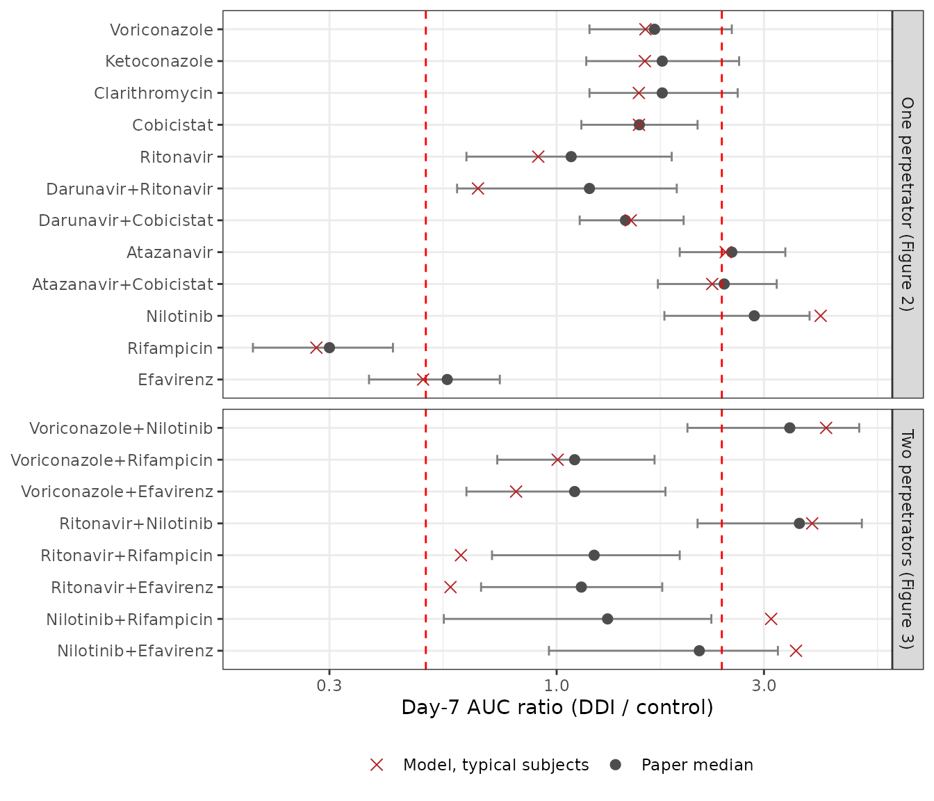
Replicates Figures 2 and 3 of Stader 2021: bictegravir day-7 AUC ratios. Bars: the paper’s median and 95% confidence interval (Table S7); points: the model’s typical subjects. Dashed lines: the efficacy-safety margin of 0.5- and 2.4-fold.
s7_sim |>
  filter(
    sex == "man", time >= 288,
    scenario %in% c("Voriconazole", "Atazanavir", "Nilotinib", "Rifampicin", "Efavirenz", "Ritonavir")
  ) |>
  ggplot(aes(time - 288, Cc, colour = arm)) +
  geom_line() +
  facet_wrap(~scenario) +
  labs(x = "Time after the seventh bictegravir dose (h)", y = "Bictegravir (ng/mL)", colour = NULL) +
  theme_bw()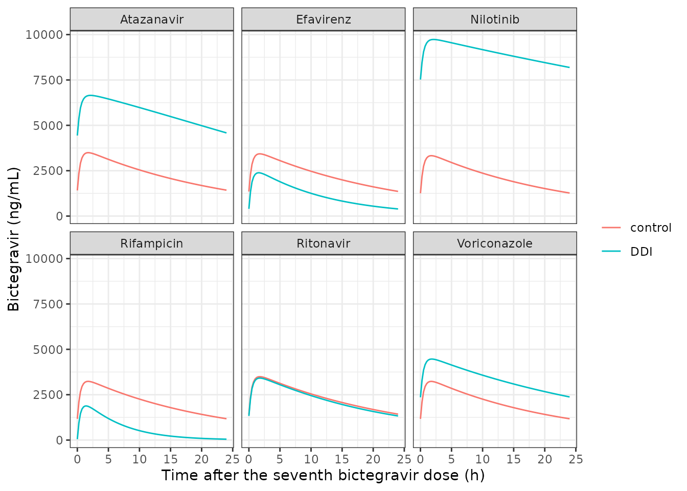
Bictegravir concentrations on the seventh day of dosing (typical man) with and without selected perpetrators.
Of the 20 scenarios, 11 reproduce the paper’s day-7 median to within 15% (the strong CYP3A inhibitors, darunavir/cobicistat, atazanavir with and without cobicistat, rifampicin, efavirenz, voriconazole with rifampicin and ritonavir with nilotinib), and all but 3 of the day-1 ratios agree to within 15%. The other nine deviate in two consistent directions. Every other nilotinib scenario (nilotinib alone and with voriconazole, rifampicin or efavirenz) gives a larger ratio than the paper: the model’s nilotinib inhibits bictegravir clearance more strongly. Ritonavir alone, darunavir with ritonavir, ritonavir with rifampicin or efavirenz, and voriconazole with efavirenz give a smaller ratio: more net induction. In every one of them the gap is larger on day 7 than on day 1. The deposited code executed in Octave behaves the same way (previous section), so the gap lies between the deposited code and the runs behind the published figures, not in this implementation; it is not resolvable from the paper or its supplements (see Assumptions and deviations).
reproduced <- c(
  "Voriconazole", "Ketoconazole", "Clarithromycin", "Cobicistat", "Darunavir+Cobicistat",
  "Atazanavir", "Atazanavir+Cobicistat", "Rifampicin", "Efavirenz",
  "Voriconazole+Rifampicin", "Ritonavir+Nilotinib"
)
larger <- c("Nilotinib", "Voriconazole+Nilotinib", "Nilotinib+Rifampicin", "Nilotinib+Efavirenz")
smaller <- c("Ritonavir", "Darunavir+Ritonavir", "Ritonavir+Rifampicin", "Ritonavir+Efavirenz", "Voriconazole+Efavirenz")
day1_checked <- c(reproduced[!grepl("\\+", reproduced)], "Ritonavir", "Voriconazole+Nilotinib", "Ritonavir+Nilotinib")
stopifnot(
  setequal(s7_ratio$scenario[abs(s7_ratio$day7_pct) < 15], reproduced),
  all(abs(s7_ratio$day1_pct[s7_ratio$scenario %in% day1_checked]) < 15),
  sum(abs(s7_ratio$day1_pct) >= 15, na.rm = TRUE) <= 3,
  # The deviating scenarios deviate in the directions described above, more
  # on day 7 than on day 1.
  all(s7_ratio$day7_pct[s7_ratio$scenario %in% larger] > 15),
  all(s7_ratio$day7_pct[s7_ratio$scenario %in% smaller] < -15),
  with(
    filter(s7_ratio, scenario %in% c(larger, smaller), !is.na(day1_pct)),
    all(abs(day7_pct) > abs(day1_pct))
  )
)
Voriconazole on its own (Table S4)
Voriconazole is one of the two drug models new in this paper, and Table S4 compares its predictions with published healthy-volunteer studies. Here the voriconazole drug file is loaded into the victim slot, without perpetrators, and single doses are simulated for the typical man; PKNCA gives Cmax, AUC0-inf and the terminal half-life, compared with the paper’s predicted means (Table S4 reports AUC to tau; for a single dose that is compared with AUC0-inf).
vori_regimens <- tibble::tribble(
  ~regimen, ~amt, ~dur, ~cmax, ~aucinf.obs, ~half.life,
  "single iv; 50 mg", 50, 2, 309, 1236, 3.9,
  "single iv; 100 mg", 100, 2, 546, 3484, 4.6,
  "single iv; 200 mg", 200, 1, 2176, 7174, 4.6,
  "single iv; 400 mg", 400, 2, 3738, 20291, 5.4,
  "single oral; 400 mg", 400, NA, 1597, 12806, 5.3
)
vori_obs <- sort(unique(c(seq(0, 4, by = 0.1), seq(4.25, 72, by = 0.25))))
vori_data <- bind_rows(lapply(seq_len(nrow(vori_regimens)), function(i) {
  r <- vori_regimens[i, ]
  dose <- if (is.na(r$dur)) {
    data.frame(time = 0, amt = r$amt, evid = 1L, cmt = "stomach", rate = 0)
  } else {
    data.frame(time = 0, amt = r$amt, evid = 1L, cmt = "venous", rate = r$amt / r$dur)
  }
  cbind(
    id = i,
    bind_rows(dose, data.frame(time = vori_obs, amt = 0, evid = 0L, cmt = "venous", rate = 0)),
    typical_subject(0), etagastric = 0,
    scenario_params("voriconazole")
  )
}))
vori_sim <- rxode2::rxSolve(mod_tv, vori_data, returnType = "data.frame", cores = 2L) |>
  mutate(regimen = vori_regimens$regimen[id])
#> ℹ omega/sigma items treated as zero: 'etahct', 'etahsa', 'etaw_adipose', 'etaw_bone', 'etaw_brain', 'etaw_gonads', 'etaw_heart', 'etaw_kidney', 'etaw_muscle', 'etaw_skin', 'etaw_thymus', 'etaw_gut', 'etaw_spleen', 'etaw_pancreas', 'etaw_liver', 'etaw_lnode', 'etaw_blood', 'etaco', 'etaltot', 'etagfr', 'etamppgl', 'etamppgl_redraw', 'etacyp3a4_liver', 'etacyp3a4_liver_redraw', 'etaugt1a1_liver', 'etaugt1a1_liver_redraw', 'etagastric', 'etasitt', 'etasitt_redraw', 'etacolt', 'etacolt_redraw', 'etacyp3a4_gut', 'etacyp3a4_gut_redraw', 'etaaag', 'etacyp2c19_liver', 'etacyp2c19_liver_redraw', 'etacyp2d6_liver', 'etacyp2d6_liver_redraw', 'etacyp2c8_liver', 'etacyp2c8_liver_redraw', 'etacyp1a2_liver', 'etacyp1a2_liver_redraw', 'etacyp2a6_liver', 'etacyp2a6_liver_redraw', 'etacyp2b6_liver', 'etacyp2b6_liver_redraw', 'etacyp2j2_liver', 'etacyp2j2_liver_redraw', 'etaugt1a4_liver', 'etaugt1a4_liver_redraw', 'etacyp2c19_gut', 'etacyp2c19_gut_redraw', 'etacyp2d6_gut', 'etacyp2d6_gut_redraw'

vori_nca <- PKNCA::pk.nca(PKNCA::PKNCAdata(
  PKNCA::PKNCAconc(filter(vori_sim, !is.na(Cc)), Cc ~ time | regimen + id),
  PKNCA::PKNCAdose(
    mutate(filter(vori_data, evid == 1), regimen = vori_regimens$regimen[id]),
    amt ~ time | regimen + id
  ),
  intervals = data.frame(start = 0, end = Inf, cmax = TRUE, aucinf.obs = TRUE, half.life = TRUE)
))

vori_cmp <- nlmixr2lib::ncaComparisonTable(
  simulated = as.data.frame(vori_nca) |> filter(PPTESTCD %in% c("cmax", "aucinf.obs", "half.life")),
  reference = select(vori_regimens, regimen, cmax, aucinf.obs, half.life),
  by = "regimen",
  units = c(cmax = "ng/mL", aucinf.obs = "ng*h/mL", half.life = "h"),
  tolerance_pct = 20
)
vori_cmp |>
  rename("Regimen" = regimen) |>
  knitr::kable(caption = paste(
    "Voriconazole single doses, typical man, versus the Table S4 predicted means.",
    "* differs by more than 20%."
))| NCA parameter | Regimen | Reference | Simulated | % diff |
|---|---|---|---|---|
| Cmax (ng/mL) | single iv; 50 mg | 309 | 761 | +146.4%* |
| Cmax (ng/mL) | single iv; 100 mg | 546 | 1600 | +193.5%* |
| Cmax (ng/mL) | single iv; 200 mg | 2180 | 4940 | +126.9%* |
| Cmax (ng/mL) | single iv; 400 mg | 3740 | 7600 | +103.3%* |
| Cmax (ng/mL) | single oral; 400 mg | 1600 | 5710 | +257.6%* |
| AUC0-∞ (obs) (ng*h/mL) | single iv; 50 mg | 1240 | 3980 | +222.1%* |
| AUC0-∞ (obs) (ng*h/mL) | single iv; 100 mg | 3480 | 8820 | +153.1%* |
| AUC0-∞ (obs) (ng*h/mL) | single iv; 200 mg | 7170 | 19200 | +168.2%* |
| AUC0-∞ (obs) (ng*h/mL) | single iv; 400 mg | 20300 | 48500 | +139.3%* |
| AUC0-∞ (obs) (ng*h/mL) | single oral; 400 mg | 12800 | 39800 | +210.6%* |
| t½ (h) | single iv; 50 mg | 3.9 | 10.6 | +170.5%* |
| t½ (h) | single iv; 100 mg | 4.6 | 10 | +117.6%* |
| t½ (h) | single iv; 200 mg | 4.6 | 10.1 | +118.8%* |
| t½ (h) | single iv; 400 mg | 5.4 | 11.5 | +112.4%* |
| t½ (h) | single oral; 400 mg | 5.3 | 11.3 | +114.0%* |
ggplot(filter(vori_sim, time <= 24), aes(time, Cc, colour = regimen)) +
  geom_line() +
  scale_y_log10() +
  labs(x = "Time (h)", y = "Voriconazole (ng/mL)", colour = NULL) +
  theme_bw()
#> Warning in scale_y_log10(): log-10 transformation introduced infinite values.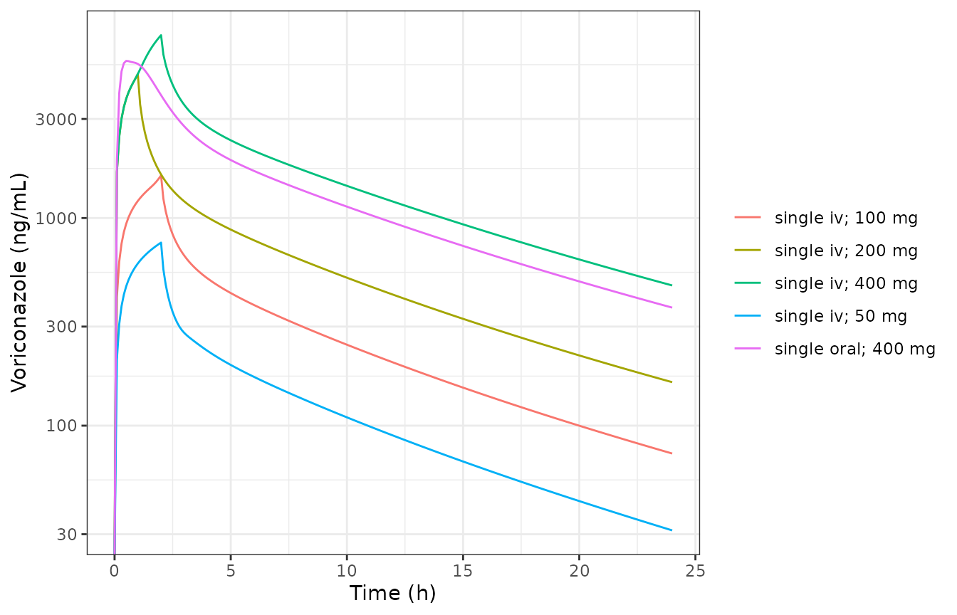
Voriconazole concentrations after single doses (typical man).
vori_auc_ratio <- as.data.frame(vori_nca) |>
  filter(PPTESTCD == "aucinf.obs") |>
  left_join(vori_regimens, by = "regimen") |>
  mutate(ratio = PPORRES / aucinf.obs)
stopifnot(all(vori_auc_ratio$ratio > 1.2))
The deposited voriconazole model gives an AUC 2.4 to 3.2 times the paper’s predicted means, although its inputs are exactly those printed in Table S1 (plus the tissue scalar below). The same happens when the deposited code itself is run (previous section, where the voriconazole concentrations are those of the Octave runs). Because voriconazole inactivates CYP3A4 almost completely at either exposure, its effect on bictegravir (Table S7) is reproduced regardless.
Assumptions and deviations
- Source. The model implements the Matlab code deposited as Supplementary Material s002. Its header reads “Publication Date: 12/12/2020, Publication: CPT - bictegravir”, and the same code is deposited with Stader et al. 2021 (doi:10.1002/cpt.2178). The implementation reproduces that code exactly (section “Check against the deposited code”).
-
Deposited code versus published results. The
deposited code does not reproduce every published prediction: the day-7
AUC ratios of the nilotinib and ritonavir-containing scenarios differ
from Table S7 (section “Prospective DDI scenarios”), and the
voriconazole exposure is higher than the Table S4 predictions (its
clearance is lower; the half-life is about twice as long). These
differences are those of the deposited code itself, possibly because the
published runs used a later revision of the code or of the drug files;
neither the paper nor the supplements allow them to be reconciled, and
the model keeps the deposited values rather than adjusting any of them.
Two single-input explanations were ruled out: neutralising the first
as-run behaviour (setting
indmax_cyp3a4to 1 for the drugs that leave it at 0) does not close the nilotinib gap, and switching off voriconazole’s own CYP3A4 inactivation does not close the voriconazole gap. - As-run behaviours kept. The four behaviours listed at the top (hepatic CYP synthesis suppression by non-inducers, drug 1’s unbound fraction in every albumin-binding term, the MPPGL CV of 2.3% when ritonavir is the last drug, and the 1-h dosing lag of ritonavir and efavirenz) are part of the deposited code and change its output, so they are kept.
-
Voriconazole tissue scalar. The voriconazole drug
file sets a global tissue-partition scalar of 2.75
(
kpscalar, citing Li et al.), which Table S1 does not list; the model uses it as deposited. -
Clarithromycin library index. Clarithromycin has a
drug file but is not registered in the framework’s drug list
(
PBPK_DefineParameters.m); it is placed after the registered drugs, which only matters for deciding which drug of a run is drug 1 (bictegravir precedes it either way). - Doses as printed. Table S3 gives voriconazole 300 mg and nilotinib 400 mg once daily (both are usually given twice daily); the scenarios use the printed regimens.
- Typical subjects. The paper simulated 100 virtual individuals per scenario; to keep the article’s run time short, each scenario is solved for a typical man and a typical woman (the generator’s mean height and weight at 35 years, every random draw at its median, gastric emptying 0.625 h). Cohorts can be drawn from the model’s random effects; see the MPPGL note above for ritonavir-last runs.
- Clinical DDI studies (Table 1, Figure 1). The bictegravir doses and sampling designs of the five clinical DDI studies (data from Gilead Sciences) are not reported, so Table 1 is not replicated.
- Reported concentration. As in the framework, the reported “plasma” concentration is the venous-blood state times the molecular weight, without a blood-to-plasma correction.