Lusutrombopag thrombopoiesis QSP (Shimizu 2021)
Source:vignettes/articles/Shimizu_2021_lusutrombopag.Rmd
Shimizu_2021_lusutrombopag.RmdModel and source
- Citation: Shimizu R, Katsube T, Wajima T. Quantitative systems pharmacology model of thrombopoiesis and platelet life-cycle, and its application to thrombocytopenia based on chronic liver disease. CPT Pharmacometrics Syst Pharmacol. 2021;10(5):489-499. doi:10.1002/psp4.12623. Model equations from Supplementary Text S1/S2 and the deposited MATLAB model code (Supplementary Model Code). Lusutrombopag PK from Katsube T et al. Clin Pharmacokinet. 2016;55:1423-1433; TPO binding kinetics from Jin F, Krzyzanski W. AAPS PharmSci. 2004;6:E9.
- Description: QSP. Thrombopoiesis and platelet life-cycle model with thrombopoietin (TPO) target-mediated disposition, driven by the oral TPO-receptor agonist lusutrombopag, in healthy adults and in thrombocytopenic patients with chronic liver disease (CLD). 27 dividing megakaryocyte progenitor compartments (26 doublings), 5 megakaryocyte maturation compartments, 9 platelet aging compartments, a 3-state TPO binding model and a 3-compartment first-order-absorption lusutrombopag PK model. TPO and unbound lusutrombopag add on one shared Emax term that scales the progenitor division rate; splenic sequestration sets the plasma fraction of the total platelet pool.
- Article: https://doi.org/10.1002/psp4.12623 (open access)
- Supplement: Supplementary Text S1 (ODEs), Text S2 (initial values), Table S1 (clinical studies) and the MATLAB model code, available from the article page.
Shimizu, Katsube and Wajima built a quantitative systems pharmacology
(QSP) model of thrombopoiesis. One megakaryocyte progenitor divides 26
times (one division per day, 27 compartments). The resulting 2^26
megakaryocytes mature through five one-day compartments and each
releases PP platelets. Platelets age through nine one-day compartments.
Endogenous thrombopoietin (TPO) follows the Jin & Krzyzanski (2004)
target-mediated disposition model, in which TPO binds the c-Mpl receptor
on platelets, so a rise in platelets lowers TPO. TPO and the
TPO-receptor agonist lusutrombopag share one Emax term that scales the
progenitor division rate kout1. Only part of the whole-body
platelet pool circulates. The rest is sequestered in the spleen (%SPS).
This split is what separates patients with chronic liver disease (CLD)
from healthy subjects. The model was not fitted to data. All values were
fixed from physiology and the literature, and the model’s predictions
were then compared with the observed lusutrombopag data.
Population
The model was applied to two populations (Methods; Supplementary Table S1):
- Healthy adults. Japanese subjects given single doses of 1, 2, 4, 10, 25 or 50 mg, non-Japanese subjects given 1 mg once daily for 14 days, and Japanese subjects given 2 mg once daily for 14 days. The baselines are TPO0 = 1.4 pM and PLT0 = 20 x 10^4/uL, with %SPS fixed at 1/3.
- Japanese patients with CLD and thrombocytopenia. These are the phase II patients, dosed at 3 mg once daily for 7 days. The baselines are TPO0 = 0.78 pM and PLT0 = 4 x 10^4/uL, with PP = 2500 platelets per megakaryocyte. %SPS follows from the steady state (78.6%).
The DIS_HEALTHY covariate selects between the two
parameter sets (1 = healthy, 0 = CLD with thrombocytopenia). The same
information is available programmatically via
readModelDb("Shimizu_2021_lusutrombopag")()$population.
Source trace
Table 1 of the paper prints two-significant-figure roundings. The
values in the model are the ones in the deposited MATLAB scripts
(initial_values_constants_*.m,
platelet_function*.m), which are what the authors
simulated.
| Equation / parameter | Value | Source location |
|---|---|---|
lka, lkel, lk12,
lk21, lk13, lk31
|
7.176, 1.358, 1.2816, 2.088, 0.03408, 0.14088 /day | Table 1 (7.2, 1.4, 1.3, 2.1, 0.034, 0.14); deposited
initial_values_constants_lusu.m
|
lvc |
13.7 L | Table 1; deposited code |
lemax |
4.52 | Table 1 (from Katsube 2019 PK/PD) |
lec50 |
183 ng/mL | Table 1 (in vitro CD34+ cells) |
lec50_tpo |
4.928 pM | Table 1 footnote b and Equation 11: (4.52 - 1) x 1.4; deposited code |
kon, koff, knf,
kfn
|
1.32 /pM/day, 60, 1.152, 3.12 /day | Table 1 (1.3, 60, 1.2, 3.1); deposited code |
kint |
2.4 /day | Text S1 (symbol only); deposited
initial_values_constants_for_platelet.m
|
rp0 |
164 pM | Table 1 Rp,0; deposited code mpl
|
lrbase_tpo_healthy, lrbase_tpo_cld
|
1.4, 0.78 pM | Table 1 TPO0 |
lrbase_plt_healthy, lrbase_plt_cld
|
20, 4 x 10^4/uL | Table 1 PLT0 |
lkout |
1 /day | Table 1 |
lpp (CLD) |
2500 | Table 1 PP; deposited CLD code |
sps_healthy |
1/3 | Text S1 (‘fixed as 1/3 in healthy subjects’); Discussion 33.3% |
eta* (4 etas) |
omega^2 = 0.1484 | Methods: ‘IIV … set at 40%’ |
d/dt(precursor1..27) |
n/a | Equations 1-2; Text S1 X1-X27 |
d/dt(mk1..5) |
n/a | Text S1 X28-X32 |
d/dt(plt1..9) |
n/a | Equations 7-8; Text S1 X33-X41 |
d/dt(tpo), tpo_ns,
tpo_complex
|
n/a | Text S1 X42-X44; deposited platelet_function*.m rows
5-7 |
PLT |
n/a | Equation 9; Text S1 ‘Platelet count in blood’ |
kout1 |
n/a | Equation 12; Text S1; floor at baseline from Methods |
| PP (healthy), %SPS (CLD) | n/a | Text S1 PP definition; Equation 10; deposited scripts |
| Initial conditions | n/a | Text S2 |
depot, central,
peripheral1/2
|
n/a | Text S1 X45-X48 |
Simulation helpers
The deposited MATLAB scripts do not give the nominal dose. They give
the nominal dose times a scenario-specific relative bioavailability
factor. The healthy 2 mg Japanese run uses
W_dose = 2000*0.857 ug. A commented-out line holds
1000*0.820*0.906*0.905 ug, which appears to be the 1 mg
non-Japanese scenario. The CLD 3 mg run uses
W_dose = 3000*0.813 ug. The factors are not explained in
the paper and presumably come from the formulation, food and population
covariates of the Katsube 2016 and 2019 lusutrombopag PK models. This
vignette applies them to amt. The model itself has no
bioavailability term.
mod <- readModelDb("Shimizu_2021_lusutrombopag")
mod_typical <- rxode2::zeroRe(mod)
#> ℹ parameter labels from comments will be replaced by 'label()'
#> Warning: No sigma parameters in the model

# One subject, once-daily oral dosing, dense observation grid on the ODE
# state `central` (algebraic outputs such as PLT, Cc and tpo come back as
# columns).
make_events <- function(amt, n_dose, healthy, t_end = 40, by = 0.05, id = 1L) {
  obs <- data.frame(
    id = id, time = seq(0, t_end, by = by), amt = 0, evid = 0L,
    cmt = "central"
  )
  dose <- data.frame(
    id = id, time = seq_len(n_dose) - 1, amt = amt, evid = 1L,
    cmt = "depot"
  )
  dplyr::bind_rows(dose, obs) |>
    dplyr::arrange(id, time, dplyr::desc(evid)) |>
    dplyr::mutate(DIS_HEALTHY = healthy)
}

peak_summary <- function(sim) {
  sim <- as.data.frame(sim)
  data.frame(
    baseline = sim$PLT[1],
    peak_increase = max(sim$PLT) - sim$PLT[1],
    tpeak = sim$time[which.max(sim$PLT)]
  )
}
Steady state without drug
The initial conditions of Text S2 put both populations at steady state. With no drug, every state must stay at its baseline. Both sides of this check use the same parameters, so the tolerance is numerical.
ss <- lapply(c(healthy = 1, cld = 0), function(h) {
  as.data.frame(rxode2::rxSolve(mod_typical, make_events(0, 1, h, t_end = 60, by = 1)))
})
#> ℹ omega/sigma items treated as zero: 'etalrbase_plt', 'etalrbase_tpo', 'etalpp', 'etalkout'
#> ℹ omega/sigma items treated as zero: 'etalrbase_plt', 'etalrbase_tpo', 'etalpp', 'etalkout'
ss_tab <- data.frame(
  population = c("Healthy", "CLD"),
  PLT_range = sapply(ss, function(s) diff(range(s$PLT))),
  TPO_range = sapply(ss, function(s) diff(range(s$tpo))),
  PLT0 = sapply(ss, function(s) s$PLT[1]),
  TPO0 = sapply(ss, function(s) s$tpo[1]),
  SPS_pct = sapply(ss, function(s) 100 * s$sps[1]),
  PP = sapply(ss, function(s) s$pp[1])
)
knitr::kable(ss_tab, digits = c(0, 10, 10, 3, 3, 2, 1), row.names = FALSE)| population | PLT_range | TPO_range | PLT0 | TPO0 | SPS_pct | PP |
|---|---|---|---|---|---|---|
| Healthy | 0e+00 | 0.00e+00 | 20 | 1.40 | 33.33 | 2483.5 |
| CLD | 7e-10 | 1.06e-08 | 4 | 0.78 | 78.56 | 2500.0 |
stopifnot(
  # Relative drift at solver-tolerance level (measured ~1e-8 for CLD TPO).
  all(ss_tab$PLT_range / ss_tab$PLT0 < 1e-6),
  all(ss_tab$TPO_range / ss_tab$TPO0 < 1e-6),
  # Discussion: %SPS 33.3% in healthy subjects and 78.6% in CLD patients.
  abs(ss_tab$SPS_pct[1] - 33.3) < 0.1,
  abs(ss_tab$SPS_pct[2] - 78.6) < 0.1
)
The derived healthy PP is 2484 platelets per megakaryocyte, consistent with the 2,500 in Table 1. The derived CLD %SPS is 78.55%, which matches the 78.6% in the Discussion.
Replicate Figure 2: healthy subjects, 14 days of once-daily dosing
fig2 <- dplyr::bind_rows(
  as.data.frame(rxode2::rxSolve(mod_typical, make_events(1 * 0.820 * 0.906 * 0.905, 14, 1))) |>
    dplyr::mutate(panel = "1 mg x 14 days (non-Japanese)"),
  as.data.frame(rxode2::rxSolve(mod_typical, make_events(2 * 0.857, 14, 1))) |>
    dplyr::mutate(panel = "2 mg x 14 days (Japanese)")
)
#> ℹ omega/sigma items treated as zero: 'etalrbase_plt', 'etalrbase_tpo', 'etalpp', 'etalkout'
#> ℹ omega/sigma items treated as zero: 'etalrbase_plt', 'etalrbase_tpo', 'etalpp', 'etalkout'
ggplot(fig2, aes(time, PLT)) +
  geom_line(colour = "darkgreen", linewidth = 1) +
  facet_wrap(~panel, scales = "free_y") +
  labs(
    x = "Time (day)", y = "Platelet count (x10^4/uL)",
    caption = "Replicates Figure 2 of Shimizu 2021 (typical-value prediction)."
  )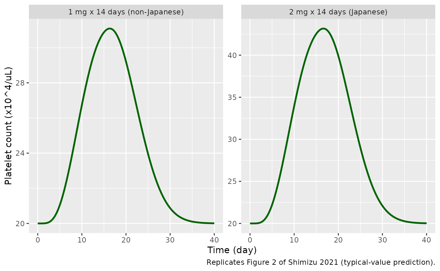
fig2_tab <- fig2 |>
  dplyr::group_by(panel) |>
  dplyr::group_modify(~ peak_summary(.x)) |>
  dplyr::ungroup() |>
  dplyr::mutate(
    published_increase = c(10.5, 23.2),
    published_tpeak = c(14.9, 16.6)
  )
fig2_tab |>
  dplyr::rename(
    Scenario = panel, "Baseline" = baseline,
    "Simulated max increase" = peak_increase, "Simulated time to peak (day)" = tpeak,
    "Published max increase" = published_increase, "Published time to peak (day)" = published_tpeak
  ) |>
knitr::kable(digits = 2)| Scenario | Baseline | Simulated max increase | Simulated time to peak (day) | Published max increase | Published time to peak (day) |
|---|---|---|---|---|---|
| 1 mg x 14 days (non-Japanese) | 20 | 11.09 | 16.30 | 10.5 | 14.9 |
| 2 mg x 14 days (Japanese) | 20 | 23.16 | 16.65 | 23.2 | 16.6 |
h2 <- fig2_tab[fig2_tab$panel == "2 mg x 14 days (Japanese)", ]
h1 <- fig2_tab[fig2_tab$panel == "1 mg x 14 days (non-Japanese)", ]
stopifnot(
  # 2 mg Japanese: the deposited script's own scenario. Reproduces the
  # Results text (23.2 x 10^4/uL at 16.6 days).
  abs(h2$peak_increase / 23.2 - 1) < 0.02,
  abs(h2$tpeak - 16.6) < 0.3,
  # 1 mg non-Japanese: the dose factor is commented out in the deposited
  # script and the non-Japanese PK is not given, so only an envelope is
  # asserted (see Assumptions and deviations).
  abs(h1$peak_increase / 10.5 - 1) < 0.10,
  abs(h1$tpeak - 14.9) < 2
)
The 2 mg Japanese scenario is the one the deposited script runs. It reproduces the reported maximum increase and time to peak. The 1 mg non-Japanese scenario gives +11.1 x 10^4/uL at day 16.3, against the published +10.5 at day 14.9. See Assumptions and deviations.
Replicate Figure 3: model components, healthy subjects, 2 mg x 14 days
fig3 <- as.data.frame(rxode2::rxSolve(mod_typical, make_events(2 * 0.857, 14, 1)))
#> ℹ omega/sigma items treated as zero: 'etalrbase_plt', 'etalrbase_tpo', 'etalpp', 'etalkout'
fig3_long <- dplyr::bind_rows(
  fig3 |> dplyr::select(time, value = tpo) |> dplyr::mutate(state = "tpo", panel = "(a) TPO (pM)"),
  fig3 |> dplyr::select(time, dplyr::all_of(paste0("precursor", 1:27))) |>
    tidyr::pivot_longer(-time, names_to = "state") |> dplyr::mutate(panel = "(b) precursor cells"),
  fig3 |> dplyr::select(time, dplyr::all_of(paste0("mk", 1:5))) |>
    tidyr::pivot_longer(-time, names_to = "state") |> dplyr::mutate(panel = "(c) megakaryocytes"),
  fig3 |> dplyr::select(time, dplyr::all_of(paste0("plt", 1:9))) |>
    tidyr::pivot_longer(-time, names_to = "state") |> dplyr::mutate(panel = "(d) platelets (whole body)")
)
ggplot(fig3_long, aes(time, value, group = state, colour = state)) +
  geom_line(show.legend = FALSE) +
  facet_wrap(~panel, scales = "free_y") +
  labs(
    x = "Time after initial dosing (day)", y = NULL,
    caption = "Replicates Figure 3 of Shimizu 2021."
  )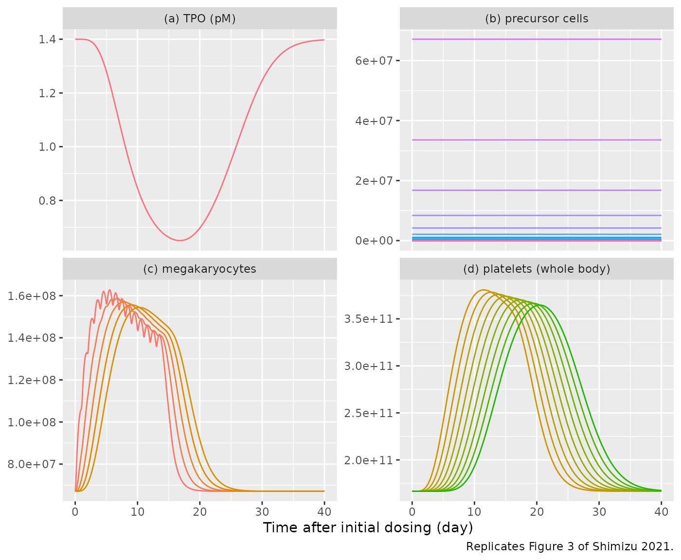
fig3_tab <- data.frame(
  quantity = c("TPO nadir (pM)", "TPO nadir time (day)", "MK1 peak (cells)", "PLT1 peak (platelets)", "PLT1 peak time (day)"),
  simulated = c(
    min(fig3$tpo), fig3$time[which.min(fig3$tpo)], max(fig3$mk1),
    max(fig3$plt1), fig3$time[which.max(fig3$plt1)]
  ),
  figure_3 = c(0.65, 17, 1.62e8, 3.8e11, 11.5)
)
fig3_tab |>
  dplyr::mutate(dplyr::across(c(simulated, figure_3), ~ signif(.x, 3))) |>
  dplyr::rename(Quantity = quantity, Simulated = simulated, "Read off Figure 3" = figure_3) |>
knitr::kable()| Quantity | Simulated | Read off Figure 3 |
|---|---|---|
| TPO nadir (pM) | 6.50e-01 | 6.50e-01 |
| TPO nadir time (day) | 1.68e+01 | 1.70e+01 |
| MK1 peak (cells) | 1.63e+08 | 1.62e+08 |
| PLT1 peak (platelets) | 3.81e+11 | 3.80e+11 |
| PLT1 peak time (day) | 1.15e+01 | 1.15e+01 |
stopifnot(
  # Values read off Figure 3 by the maintainers (+/- one gridline fraction).
  abs(fig3_tab$simulated[1] / 0.65 - 1) < 0.05,
  abs(fig3_tab$simulated[2] - 17) < 1,
  abs(fig3_tab$simulated[3] / 1.62e8 - 1) < 0.05,
  abs(fig3_tab$simulated[4] / 3.8e11 - 1) < 0.05,
  # Precursor counts are unaffected by the drug (Results).
  diff(range(fig3$precursor27)) < 1e-3 * 2^26
)
The simulation reproduces what the paper describes. TPO falls as platelets rise, because more receptors bind it. The precursor compartments do not change. Megakaryocytes and platelets rise in turn along the chain.
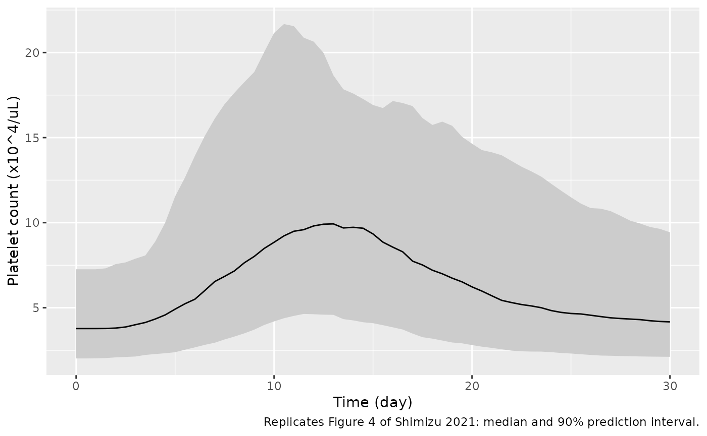
Replicate Figure 4: CLD patients, 3 mg x 7 days (virtual cohort)
The authors simulated 200 virtual patients in NONMEM. They resampled patient demographics, drew PK variability from Katsube 2019, and set 40% IIV on PLT0, TPO0, PP and kout. Neither the patient data nor the NONMEM code is public. The cohort below keeps the 40% IIV on the four PD parameters and uses typical-value PK.
rxode2::rxSetSeed(2021)
n_sub <- 200
ev_cld <- dplyr::bind_rows(lapply(seq_len(n_sub), function(i) {
  make_events(3 * 0.813, 7, 0, t_end = 30, by = 0.5, id = i)
}))
sim_cld <- as.data.frame(rxode2::rxSolve(mod, ev_cld))
#> ℹ parameter labels from comments will be replaced by 'label()'

vpc <- sim_cld |>
  dplyr::group_by(time) |>
  dplyr::summarise(
    Q05 = quantile(PLT, 0.05), Q50 = median(PLT), Q95 = quantile(PLT, 0.95),
    .groups = "drop"
  )
ggplot(vpc, aes(time, Q50)) +
  geom_ribbon(aes(ymin = Q05, ymax = Q95), fill = "grey80") +
  geom_line() +
  labs(
    x = "Time (day)", y = "Platelet count (x10^4/uL)",
    caption = "Replicates Figure 4 of Shimizu 2021: median and 90% prediction interval."
  )
per_sub <- sim_cld |>
  dplyr::group_by(id) |>
  dplyr::summarise(
    baseline = PLT[time == 0][1], peak = max(PLT), tpeak = time[which.max(PLT)],
    fplasma = 1 - sps[1], .groups = "drop"
  )
typ_cld <- peak_summary(rxode2::rxSolve(mod_typical, make_events(3 * 0.813, 7, 0)))
#> ℹ omega/sigma items treated as zero: 'etalrbase_plt', 'etalrbase_tpo', 'etalpp', 'etalkout'
cld_tab <- data.frame(
  quantity = c(
    "Typical-value max increase", "Typical-value time to peak (day)",
    "Cohort median baseline", "Cohort median of peak / baseline",
    "Cohort median time to peak (day)"
  ),
  simulated = c(
    typ_cld$peak_increase, typ_cld$tpeak, median(per_sub$baseline),
    median(per_sub$peak / per_sub$baseline), median(per_sub$tpeak)
  ),
  published = c(3.39, 12.9, 3.4, 2.4, 12.9)
)
knitr::kable(cld_tab, digits = 2)| quantity | simulated | published |
|---|---|---|
| Typical-value max increase | 7.21 | 3.39 |
| Typical-value time to peak (day) | 13.10 | 12.90 |
| Cohort median baseline | 3.78 | 3.40 |
| Cohort median of peak / baseline | 2.80 | 2.40 |
| Cohort median time to peak (day) | 13.00 | 12.90 |
stopifnot(
  # Typical-value CLD run: same parameters as the deposited CLD script, so
  # this is deterministic.
  abs(typ_cld$tpeak - 12.9) < 0.5,
  # Cohort statistics: assert on the centre with room for the draw.
  abs(median(per_sub$baseline) / 4 - 1) < 0.15,
  abs(median(per_sub$tpeak) - 12.9) < 1.5,
  median(per_sub$peak / per_sub$baseline) > 2,
  median(per_sub$peak / per_sub$baseline) < 3.5
)
The time to peak agrees with the paper (13.1 days typical, against 12.9 days reported). The magnitude does not agree with the text. The Results report a “maximum increase” of 3.39 x 10^4/uL. The typical-value run of the deposited CLD script gives +7.2 x 10^4/uL, and so does this model, which is identical to that script. The published 3.39 matches the day-0 median of Figure 4 (about 3.4). The Figure 4 median line then rises to about 8.3 x 10^4/uL, an increase of about 4.9 and a peak-to-baseline ratio of about 2.4. The ratio here is about 2.8. The remaining gap is consistent with the NONMEM simulation’s resampled patient baselines and Katsube 2019 PK variability, neither of which is available. The published column of the table gives the text value for the typical-value rows and values read off Figure 4 for the cohort rows.
Because PP and PLT0 both carry IIV, about 1% of virtual CLD patients
draw a plasma fraction 1 - %SPS above 1 (a negative splenic
pool). This cohort has 2 such patients. The paper does not say how its
NONMEM simulation handled this case. The model does not constrain
it.
PKNCA validation of the lusutrombopag PK
The paper reports no NCA. The check below confirms the PK layer by identity: for single doses of 1, 2 and 4 mg, AUC0-inf x kel x Vc must equal the dose. The PK has no variability and does not depend on the platelet model.
pk_events <- dplyr::bind_rows(lapply(seq_along(c(1, 2, 4)), function(i) {
  dose <- c(1, 2, 4)[i]
  obs_t <- sort(unique(c(seq(0, 2, by = 0.02), seq(2, 30, by = 0.25), seq(30, 400, by = 2))))
  dplyr::bind_rows(
    data.frame(id = i, time = 0, amt = dose, evid = 1L, cmt = "depot"),
    data.frame(id = i, time = obs_t, amt = 0, evid = 0L, cmt = "central")
  ) |>
    dplyr::mutate(DIS_HEALTHY = 1, treatment = paste(dose, "mg"))
}))
sim_pk <- as.data.frame(rxode2::rxSolve(mod_typical, pk_events, keep = "treatment"))
#> ℹ omega/sigma items treated as zero: 'etalrbase_plt', 'etalrbase_tpo', 'etalpp', 'etalkout'

sim_nca <- sim_pk |>
  dplyr::filter(!is.na(Cc)) |>
  dplyr::select(id, time, Cc, treatment)
sim_nca <- dplyr::bind_rows(
  sim_nca,
  sim_nca |> dplyr::distinct(id, treatment) |> dplyr::mutate(time = 0, Cc = 0)
) |>
  dplyr::distinct(id, treatment, time, .keep_all = TRUE) |>
  dplyr::arrange(id, treatment, time)

dose_df <- pk_events |>
  dplyr::filter(evid == 1) |>
  dplyr::select(id, time, amt, treatment)

conc_obj <- PKNCA::PKNCAconc(sim_nca, Cc ~ time | treatment + id)
dose_obj <- PKNCA::PKNCAdose(dose_df, amt ~ time | treatment + id)
intervals <- data.frame(start = 0, end = Inf, cmax = TRUE, tmax = TRUE, aucinf.obs = TRUE)
nca_res <- PKNCA::pk.nca(PKNCA::PKNCAdata(conc_obj, dose_obj, intervals = intervals))

nca_wide <- as.data.frame(nca_res$result) |>
  dplyr::filter(PPTESTCD %in% c("cmax", "tmax", "aucinf.obs")) |>
  dplyr::select(treatment, PPTESTCD, PPORRES) |>
  tidyr::pivot_wider(names_from = PPTESTCD, values_from = PPORRES) |>
  dplyr::mutate(
    dose = as.numeric(sub(" mg", "", treatment)),
    # Units: dose in mg, AUC in ng*day/mL, kel in 1/day, Vc in L.
    expected_auc = 1000 * dose / (1.358 * 13.7),
    pct_diff = 100 * (aucinf.obs / expected_auc - 1)
  )
nca_wide |>
  dplyr::select(treatment, cmax, tmax, aucinf.obs, expected_auc, pct_diff) |>
  dplyr::rename(
    Treatment = treatment, "Cmax (ng/mL)" = cmax, "Tmax (day)" = tmax,
    "AUC0-inf (ng*day/mL)" = aucinf.obs, "Dose/(kel*Vc) (ng*day/mL)" = expected_auc,
    "Difference (%)" = pct_diff
  ) |>
knitr::kable(digits = 3)| Treatment | Cmax (ng/mL) | Tmax (day) | AUC0-inf (ng*day/mL) | Dose/(kelVc) (ngday/mL) | Difference (%) |
|---|---|---|---|---|---|
| 1 mg | 41.845 | 0.24 | 53.733 | 53.750 | -0.032 |
| 2 mg | 83.690 | 0.24 | 107.466 | 107.500 | -0.032 |
| 4 mg | 167.380 | 0.24 | 214.933 | 215.001 | -0.032 |
Assumptions and deviations
- Deposited code over Table 1 roundings. Table 1 rounds the rate constants to two significant figures (for example kon 1.3, knf 1.2, ka 7.2). The model uses the values in the deposited MATLAB scripts (kon 1.32, knf 1.152, ka 7.176 and so on), because those produced the published figures.
-
kintis not in the paper. Text S1 names the internalization rate of the TPO-receptor complex but does not give its value. It is taken from the deposited scripts: 2.4 /day for healthy subjects, and 2.4 x 0.78/1.4 for CLD patients. -
Population scaling of
kintand Rp,0. The Methods say every CLD parameter other than TPO0, PLT0 and PP equals the healthy value. The deposited CLD script, however, scales kint by TPO0/1.4 and Rp,0 by PLT0/20. The model follows the script and applies both scalings to the individual baselines, which is the identity for a typical healthy subject. This matters only when TPO0 or PLT0 varies between subjects. -
Text S1 vs the code for receptor binding. Text S1
writes the binding term as
kon * TPO * Rp,0 * PLT. The deposited code, which is what was run, normalises by the baseline:kon * TPO * Rp,0 * PLT/PLT0. The model follows the code. - Unbound fraction. Equation 12 multiplies both the lusutrombopag concentration and EC50Lusu by fuLusu (0.1%), so it cancels. The deposited code omits it, and so does the model.
-
Floor on
kout1. The Methods restrict kout1 to its initial value or higher (1 /day for healthy subjects, 0.62 /day for CLD). The model writes this askout * Emax * TPO0/(EC50TPO + TPO0), which gives exactly those values for both populations at typical parameters. - Healthy PP derivation. For healthy subjects the splenic fraction is fixed at 1/3 and PP is derived. The model includes the baseline TPO effect (which equals 1 at the healthy TPO0) in that derivation, so the steady state also holds when TPO0 varies.
-
Dose-scaling factors. The deposited scripts
multiply the nominal dose by 0.857 (2 mg healthy Japanese), 0.820 x
0.906 x 0.905 (commented out, apparently 1 mg non-Japanese) and 0.813 (3
mg CLD). This vignette applies them to
amt. They appear to be relative bioavailability factors from the Katsube 2016 and 2019 PK models, which the paper does not print. - 1 mg non-Japanese scenario. The model gives +11.1 x 10^4/uL at day 16.3, against +10.5 at day 14.9 in the paper. The non-Japanese PK covariates behind that simulation are not in the paper.
- CLD Figure 4. Neither the NONMEM simulation (resampled demographics, Katsube 2019 PK variability) nor the patient data are available. The cohort here uses typical-value PK and the stated 40% IIV on PLT0, TPO0, PP and kout. The text’s “maximum increase 3.39 x 10^4/uL” does not match the deposited CLD script (+7.2) and appears to be the day-0 median of Figure 4. See the Figure 4 section.
-
IIV encoding. The paper’s “40%” IIV is encoded as a
log-normal variance of log(1 + 0.4^2) = 0.1484. The etas are used only
for the CLD simulation. The healthy-subject simulations in the paper are
typical-value runs, so use
rxode2::zeroRe()for them.etalpphas no effect whenDIS_HEALTHY = 1, because PP is then derived. - No residual error. The paper simulates only, with no fitted residual error, so the model has none.
- Global sensitivity analysis. Figure 5 (Sobol indices) comes from MATLAB’s GSAT toolbox. It is not reproduced here.