Dolutegravir pediatric weight-band dosing (Chandasana 2023)
Source:vignettes/articles/Chandasana_2023_dolutegravir.Rmd
Chandasana_2023_dolutegravir.RmdModel and source
#> ℹ parameter labels from comments will be replaced by 'label()'
#> Warning: some etas defaulted to non-mu referenced, possible parsing error: etaiov_lcl_1, etaiov_lcl_2, etaiov_lcl_3, etaiov_lcl_4, etaiov_lka_1, etaiov_lka_2
#> as a work-around try putting the mu-referenced expression on a simple line
Citation: Chandasana H, Thapar M, Hayes S, Baker M, Gibb DM, Turkova A, Ford D, Ruel T, Wiznia A, Fairlie L, Bwakura-Dangarembizi M, Mujuru H, Alvero C, Farhad M, Hazra R, Townley E, Buchanan A, Bollen P, Waalewijn H, Colbers A, Burger D, Acosta EP, Singh R; for the IMPAACT P1093, ODYSSEY (PENTA 20) Study Teams. Population pharmacokinetic modeling of dolutegravir to optimize pediatric dosing in HIV-1-infected infants, children, and adolescents. Clin Pharmacokinet. 2023;62(10):1445-1459. doi:10.1007/s40262-023-01289-5. Structural equations, parameter estimates and the full random-effects covariance are taken from Chandasana 2023 Table 2 and from the final NONMEM control stream reproduced verbatim in Supplementary Text 1 of the Electronic Supplementary Material. The same fit was later applied without re-estimation to the abacavir/dolutegravir/lamivudine fixed-dose combination in IMPAACT 2019; see modellib(‘Chandasana_2024b_dolutegravir’).
Description: One-compartment oral population PK model with first-order absorption and elimination, estimated allometric weight scaling on CL/F and V/F, a fixed postmenstrual-age enzyme-maturation function on CL/F, formulation-specific absorption rate constant and formulation- and food-specific relative bioavailability for dolutegravir in infants, children and adolescents with HIV-1 pooled from IMPAACT P1093 and ODYSSEY (Chandasana 2023)
Supplement (Electronic Supplementary Material, includes the final NONMEM control stream as Supplementary Text 1): https://static-content.springer.com/esm/art%3A10.1007%2Fs40262-023-01289-5/MediaObjects/40262_2023_1289_MOESM1_ESM.docx
Chandasana 2023 pooled the IMPAACT P1093 and ODYSSEY (PENTA 20) pediatric dolutegravir trials into a single population PK model, and used it to confirm the WHO weight-band doses for infants, children and adolescents down to 4 weeks of age and 3 kg. This vignette reproduces the simulated steady-state exposures of the paper’s Table 3 and checks the model against the paper’s own printed derived quantities.
Population
The analysis pooled 239 participants – 151 from IMPAACT P1093 (a phase I/II multicentre open-label single-arm trial in children and adolescents aged 4 weeks to <18 years) and 88 from ODYSSEY (a phase II/III multicentre open-label randomised non-inferiority trial in children aged at least 28 days and <18 years). 240 participants provided 2714 plasma concentrations, of which 64 were excluded (21 below the limit of quantification, 7 outliers or very low concentrations, 4 sample mix-ups, 13 haemolysed samples, 6 for non-adherence and 13 from one participant with multiple co-morbidities), leaving 2650 samples (1909 intensive and 741 sparse) from 239 participants (Chandasana 2023 Sect. 3.1).
Baseline age ranged from 0.170 to 17.5 years (median 6.00), baseline weight from 3.9 to 91.0 kg, the cohort was 49.8% female, and 79.5% were Black – the ODYSSEY cohort being 100% Black (Chandasana 2023 Table 1). Dolutegravir was given once daily under fasting conditions as film-coated tablets, dispersible tablets or granules for oral suspension across the WHO weight bands.
The same information is available programmatically via
readModelDb("Chandasana_2023_dolutegravir")()$population.
Source trace
The per-parameter origin is recorded as an in-file comment next to
each ini() entry in
inst/modeldb/specificDrugs/Chandasana_2023_dolutegravir.R.
The table below collects them in one place for review. “Control stream”
refers to the final NONMEM model code reproduced verbatim as
Supplementary Text 1 of the Electronic Supplementary Material.
| Equation / parameter | Value | Source location |
|---|---|---|
lcl (CL/F at 70 kg, FMAT = 1) |
1.03 L/h (95% CI 0.980-1.07) | Table 2 |
lvc (V/F at 70 kg) |
13.6 L (95% CI 13.0-14.3) | Table 2 |
lka (Ka, film-coated tablet) |
0.854 1/h (95% CI 0.686-1.06) | Table 2 |
e_form_dt_ka (Ka ratio, DT / granules) |
2.04 (95% CI 1.41-2.67); product 0.854 x 2.04 = 1.74 1/h | Table 2; covariate-relationship block; Table S1 |
e_wt_cl |
0.455 (95% CI 0.418-0.492) | Table 2 |
e_wt_vc |
0.556 (95% CI 0.514-0.598) | Table 2 |
tmat50 |
52.2 postmenstrual weeks, FIX | Table 2 (footnote a; Anderson & Holford 2009); control stream
THETA(8)
|
hill_mat |
3.43, FIX | Table 2 (footnote a); control stream THETA(7)
|
e_food_fdepot (without regard to food) |
1.10 (95% CI 1.03-1.17) | Table 2; control stream THETA(4)
|
e_form_dt_fdepot (DT / granules) |
1.53 (95% CI 1.43-1.63) | Table 2; control stream THETA(9)
|
IIV block etalcl, etalvc,
etalka
|
var 0.0863 / 0.0698 / 0.762; cov 0.0499, 0.0953, 0.138 | Table 2; control stream $OMEGA BLOCK(3)
|
etaiov_lcl_1..4 |
0.115 each (CV 33.9%) | Table 2 (four rows); control stream $OMEGA BLOCK(1) +
SAME(3)
|
etaiov_lka_1..2 |
0.610 each (CV 91.7%) | Table 2 (two rows); control stream $OMEGA BLOCK(1) +
SAME(1)
|
propSd / addSd (P1093) |
var 0.0818 / 0.00164, i.e. CV 28.6% and SD 0.0405 ug/mL | Table 2 |
propSd_odyssey / addSd_odyssey
|
var 0.0123 / 0.0900, i.e. CV 11.1% and SD 0.300 ug/mL | Table 2 |
FMAT = PMA^Hill / (PMA^Hill + TM50^Hill),
PMA = PNA*52 + 40
|
n/a | Covariate-relationship block under Table 2; control stream
$PK
|
CL/F = 1.03 * (WT/70)^0.455 * FMAT,
V/F = 13.6 * (WT/70)^0.556
|
n/a | Covariate-relationship block under Table 2 |
F1 = 1 * 1.10^SFLAG * 1.53^FFLAG |
n/a | Control stream $PK (with its own comment block
enumerating the four combinations); Table S1 |
| One-compartment first-order absorption and elimination | n/a | Sect. 3.2; control stream
$SUBROUTINES ADVAN2 TRANS2
|
| Combined proportional + additive error, per study | n/a | Control stream $ERROR
|
The two effects that are ratios, not absolute values
Two rows of Table 2 are easy to misread, and both are settled unambiguously by the control stream and by Table S1:
-
KA~DT and granules = 2.04is a multiplier, not a Ka. The control stream formsKAFORM = THETA(17)**FORMKandKA = EXP(MU_3 + ETA(3)) * IOVKA * KAFORM. The dispersible-tablet Ka is therefore0.854 x 2.04 = 1.74 1/h, which the paper spells out in the covariate-relationship block and tabulates in Table S1 as 1.74 (95% CI 1.20-2.28). -
The 1.10 food effect is not
film-coated-tablet-specific. The control stream forms
F1 = 1 * THETA(4)**SFLAG * THETA(9)**FFLAG, and its own comments enumerate fasted FCT = 1, fasted DT =THETA(9), fed FCT =THETA(4), fed DT =THETA(9) * THETA(4). Table S1 accordingly gives F for the dispersible tablet without regard to food as 1.68 = 1.10 x 1.53. Table 2 lists a fed estimate on the FCT row only because that row is the reference level.
Both are checked numerically below.
Errata noted while transcribing
- Sect. 3.2 prints the weight exponent on V/F as 0.566, while Table 2 gives 0.556 with a 95% CI of 0.514-0.598 that is centred on 0.556. Table S1 also gives 0.556. The tabulated value is used.
- The covariate-relationship block prints the confidence interval for F without regard to food, DT/granules as “1.68 (1.47-0.91)”. The upper bound is a transposition: the stated arithmetic is 1.03 x 1.43 = 1.47 to 1.17 x 1.63 = 1.91. Only the point estimate 1.68 enters the model.
- Table 3’s Cmax column is not mutually consistent with its own AUC0-24 column under the published model: in 8 of the 11 QD arms the reported median Cmax exceeds the largest value attainable at an infinite absorption rate given the reported median AUC0-24, and the remaining 3 sit within 3% of that ceiling. This is demonstrated numerically below. The AUC0-24 and C24 columns are consistent with each other and with the model, and are reproduced here.
-
Table 1’s categorical counts do not sum to the column
N (e.g. metal-cation products “Absent 123 (81.5)” plus “Present
45 (29.8)” for N = 151). These are time-varying flags counted per record
rather than mutually exclusive per-subject categories. No model
parameter depends on them – every covariate outside weight, age,
formulation and food was fixed to no effect in the final model
(
THETA(10)-THETA(16)are all0 FIXor1 FIX).
Deterministic checks against the paper’s printed derived quantities
Before simulating a cohort, confirm the packaged model reproduces the four derived quantities the paper prints for itself. These are exact algebraic identities, so they are asserted tightly.
mod <- readModelDb("Chandasana_2023_dolutegravir")
ini_tbl <- ui$iniDf
th <- function(nm) ini_tbl$est[match(nm, ini_tbl$name)]

ka_fct    <- exp(th("lka"))
ka_dt     <- exp(th("lka") + th("e_form_dt_ka"))
f_fct_fed <- exp(th("e_food_fdepot"))
f_dt_fast <- exp(th("e_form_dt_fdepot"))
f_dt_fed  <- exp(th("e_food_fdepot") + th("e_form_dt_fdepot"))

derived <- tibble::tibble(
  Quantity  = c("Ka, film-coated tablet (1/h)",
                "Ka, dispersible tablet / granules (1/h)",
                "F, film-coated tablet without regard to food",
                "F, fasted dispersible tablet / granules",
                "F, dispersible tablet / granules without regard to food"),
  Model     = c(ka_fct, ka_dt, f_fct_fed, f_dt_fast, f_dt_fed),
  Published = c(0.854, 1.74, 1.10, 1.53, 1.68),
  Source    = c("Table 2", "Covariate block / Table S1", "Table 2",
                "Table 2", "Covariate block / Table S1")
) |>
  dplyr::mutate(`% difference` = 100 * (Model - Published) / Published)

knitr::kable(derived, digits = c(0, 3, 3, 0, 2),
caption = "Model-derived formulation and food effects vs the values Chandasana 2023 prints for itself.")| Quantity | Model | Published | Source | % difference |
|---|---|---|---|---|
| Ka, film-coated tablet (1/h) | 0.854 | 0.854 | Table 2 | 0.00 |
| Ka, dispersible tablet / granules (1/h) | 1.742 | 1.740 | Covariate block / Table S1 | 0.12 |
| F, film-coated tablet without regard to food | 1.100 | 1.100 | Table 2 | 0.00 |
| F, fasted dispersible tablet / granules | 1.530 | 1.530 | Table 2 | 0.00 |
| F, dispersible tablet / granules without regard to food | 1.683 | 1.680 | Covariate block / Table S1 | 0.18 |
# Exact algebra against printed 3-significant-figure values: the only slack is
# the paper's own rounding, so 0.5% is generous and a mis-encoded ratio (e.g.
# 2.04 read as an absolute Ka) would show up as a 17% or 134% miss.
stopifnot(max(abs(derived$`% difference`)) < 0.5)
The maturation function is likewise checked against the two
statements the paper makes about it: TM50 is 52.2
postmenstrual weeks, which the paper equates to 12 weeks of postnatal
age, and FMAT must be at half of its maximum there.
pma_weeks <- function(pna_years) pna_years * 52 + 40
fmat <- function(pma_wk) pma_wk^th("hill_mat") / (pma_wk^th("hill_mat") + th("tmat50")^th("hill_mat"))

# 12 weeks postnatal = 12/52 years -> PMA = 52 weeks; TM50 = 52.2 weeks.
stopifnot(abs(pma_weeks(12 / 52) - 52) < 1e-9)
stopifnot(abs(fmat(th("tmat50")) - 0.5) < 1e-12)
# Maturation is essentially complete by school age (FMAT = 0.9986 at 6 years)
# and all but exact in adolescence (0.99996 at 18 years). Deterministic
# algebra, so these bounds sit just under the exact values.
stopifnot(fmat(pma_weeks(6)) > 0.998, fmat(pma_weeks(18)) > 0.9999)
# ...and materially incomplete in a young infant, which is what separates the
# 10 mg (<6 months) and 15 mg (>=6 months) doses in the 6-10 kg band.
stopifnot(fmat(pma_weeks(2 / 12)) < 0.55, fmat(pma_weeks(9 / 12)) > 0.75)
Virtual cohort
Original observed data are not publicly available. Chandasana 2023 Sect. 2.4 simulated 200 participants (100 male, 100 female) for each of 11 weight band / dose / formulation combinations, sampling age uniformly from the relevant CDC growth chart and deriving each subject’s weight from that chart. The cohort below mirrors that design at the same 200 participants per arm: age is drawn uniformly over the age window implied by each band, weight is taken from a piecewise-linear interpolation of the CDC 2000 sex-averaged 50th-percentile weight-for-age curve with lognormal scatter, and the result is clamped into the band the arm is defined by.
# rxSetSeed fixes rxode2's RNG per solver thread, not across thread counts, so
# CI draws a different cohort than a workstation does. Every assertion below is
# written to hold for any cohort this model can produce (see the notes on each).
rxode2::rxSetSeed(20230821)
set.seed(20230821)

# CDC 2000 50th-percentile weight-for-age, sexes averaged. Reference data for
# constructing the virtual cohort only -- NOT a model parameter, and not taken
# from Chandasana 2023.
cdc_age_yr <- c(1, 2, 3, 4, 6, 9, 12, 18, 24) / 12
cdc_wt_kg  <- c(4.4, 5.5, 6.3, 7.0, 7.9, 9.0, 9.9, 11.3, 12.5)
cdc_age_yr <- c(cdc_age_yr, 3:18)
cdc_wt_kg  <- c(cdc_wt_kg, 14.3, 16.3, 18.3, 20.7, 23.2, 26.0, 29.2, 32.7,
                36.7, 41.3, 46.0, 50.6, 54.6, 58.0, 60.6, 62.6)
cdc_weight_for_age <- function(age_yr) {
  stats::approx(cdc_age_yr, cdc_wt_kg, xout = age_yr, rule = 2)$y
}

# The 11 QD weight band / dose / formulation combinations of Chandasana 2023
# Table 3. Age windows are those the paper attaches to each band (Table 3 and
# Sect. 3.4); where a band carries no explicit age, the window is the age range
# over which the CDC median weight falls inside the band.
bands <- tibble::tribble(
  ~arm,                            ~wt_lo, ~wt_hi, ~age_lo, ~age_hi, ~form, ~dose,
  "3 to <6 kg (>=1 month), DT 5",     3.0,    6.0,  1/12,     4/12,  "DT",   5,
  "6 to <10 kg (1-<6 mo), DT 10",     6.0,   10.0,  1/12,     6/12,  "DT",  10,
  "6 to <10 kg (>=6 mo), DT 15",      6.0,   10.0,  6/12,     2.0,   "DT",  15,
  "10 to <14 kg, DT 20",             10.0,   14.0,  1.0,      4.0,   "DT",  20,
  "14 to <20 kg, DT 25",             14.0,   20.0,  3.0,      6.0,   "DT",  25,
  "14 to <20 kg, FCT 40",            14.0,   20.0,  3.0,      6.0,   "FCT", 40,
  "20 to <25 kg, DT 30",             20.0,   25.0,  5.5,      8.0,   "DT",  30,
  "20 to <25 kg, FCT 50",            20.0,   25.0,  5.5,      8.0,   "FCT", 50,
  "25 to <30 kg, FCT 50",            25.0,   30.0,  7.5,      9.5,   "FCT", 50,
  "30 to <35 kg, FCT 50",            30.0,   35.0,  9.0,     11.0,   "FCT", 50,
  ">=35 kg, FCT 50",                 35.0,   90.0, 11.0,     18.0,   "FCT", 50
)

n_per_arm <- 200L
n_doses   <- 14L            # 14 QD doses, i.e. > 20 elimination half-lives
t_last    <- 24 * (n_doses - 1L)

# Observation grid over the final dosing interval: fine through absorption so
# Cmax and Tmax are resolved, coarser through the terminal phase.
obs_grid <- sort(unique(c(seq(0, 6, by = 0.1), seq(6, 24, by = 0.5))))

make_arm <- function(row, id_offset) {
  age_yr <- stats::runif(n_per_arm, row$age_lo, row$age_hi)
  wt <- cdc_weight_for_age(age_yr) * exp(stats::rnorm(n_per_arm, 0, 0.12))
  wt <- pmin(pmax(wt, row$wt_lo), row$wt_hi)
  subj <- tibble::tibble(
    id  = id_offset + seq_len(n_per_arm),
    arm = row$arm,
    WT  = wt,
    # The model's PAGE column is postmenstrual age in MONTHS; the source model
    # works in postmenstrual WEEKS with PMA = PNA(years) * 52 + 40, so convert
    # back through the same 4.348125 weeks-per-month factor model() applies.
    PAGE          = (age_yr * 52 + 40) / 4.348125,
    FORM_DTG_DT   = as.numeric(row$form == "DT"),
    FED           = 0,      # dosed fasted, as in P1093 and ODYSSEY
    STUDY_ODYSSEY = 0,
    OCC           = 1,      # single steady-state occasion
    dose_mg       = row$dose
  )
  doses <- subj |>
    dplyr::mutate(time = 0, amt = dose_mg, evid = 1L, cmt = "depot",
                  addl = n_doses - 1L, ii = 24)
  obs <- subj |>
    tidyr::crossing(tad = obs_grid) |>
    dplyr::mutate(time = t_last + tad, amt = NA_real_, evid = 0L,
                  cmt = "central", addl = 0L, ii = 0)
  dplyr::bind_rows(doses, obs) |> dplyr::arrange(id, time, dplyr::desc(evid))
}

events <- do.call(
  dplyr::bind_rows,
  lapply(seq_len(nrow(bands)), function(i) {
    make_arm(bands[i, ], id_offset = (i - 1L) * n_per_arm)
  })
)

stopifnot(nrow(dplyr::distinct(events, id)) == n_per_arm * nrow(bands))
stopifnot(!anyDuplicated(unique(events[, c("id", "time", "evid")])))| Weight band / dose | N | Dose (mg) | Formulation | Weight (kg), median | Weight (kg), range | Age (y), median |
|---|---|---|---|---|---|---|
| 3 to <6 kg (>=1 month), DT 5 | 200 | 5 | DT | 5.8 | 3.6-6 | 0.21 |
| 6 to <10 kg (1-<6 mo), DT 10 | 200 | 10 | DT | 6.5 | 6-10 | 0.28 |
| 6 to <10 kg (>=6 mo), DT 15 | 200 | 15 | DT | 10.0 | 7-10 | 1.18 |
| 10 to <14 kg, DT 20 | 200 | 20 | DT | 13.2 | 10-14 | 2.51 |
| 14 to <20 kg, DT 25 | 200 | 25 | DT | 17.3 | 14-20 | 4.43 |
| 14 to <20 kg, FCT 40 | 200 | 40 | FCT | 17.3 | 14-20 | 4.62 |
| 20 to <25 kg, DT 30 | 200 | 30 | DT | 22.5 | 20-25 | 6.75 |
| 20 to <25 kg, FCT 50 | 200 | 50 | FCT | 22.0 | 20-25 | 6.73 |
| 25 to <30 kg, FCT 50 | 200 | 50 | FCT | 27.4 | 25-30 | 8.39 |
| 30 to <35 kg, FCT 50 | 200 | 50 | FCT | 32.3 | 30-35 | 9.97 |
| >=35 kg, FCT 50 | 200 | 50 | FCT | 51.1 | 35-74.4 | 14.78 |
Simulation
sim <- rxode2::rxSolve(
  mod, events = events,
  keep = c("arm", "WT", "PAGE", "dose_mg", "FORM_DTG_DT")
) |>
  as.data.frame() |>
  # rxSolve returns observation records only, so no evid filter is needed (and
  # `evid` is not among the returned columns); restrict to the final interval.
  dplyr::filter(time >= t_last) |>
  dplyr::mutate(tad = time - t_last)
#> ℹ parameter labels from comments will be replaced by 'label()'
#> Warning: some etas defaulted to non-mu referenced, possible parsing error: etaiov_lcl_1, etaiov_lcl_2, etaiov_lcl_3, etaiov_lcl_4, etaiov_lka_1, etaiov_lka_2
#> as a work-around try putting the mu-referenced expression on a simple line

stopifnot(nrow(sim) == n_per_arm * nrow(bands) * length(obs_grid))
Steady-state concentration-time profiles
sim |>
  dplyr::group_by(arm, tad) |>
  dplyr::summarise(Q10 = stats::quantile(Cc, 0.10),
                   Q50 = stats::quantile(Cc, 0.50),
                   Q90 = stats::quantile(Cc, 0.90),
                   .groups = "drop") |>
  dplyr::mutate(arm = factor(arm, levels = bands$arm)) |>
  ggplot(aes(tad, Q50)) +
  geom_ribbon(aes(ymin = Q10, ymax = Q90), alpha = 0.25) +
  geom_line() +
  geom_hline(yintercept = 0.995, colour = "red", linetype = "dashed") +
  geom_hline(yintercept = 0.697, colour = "blue", linetype = "dashed") +
  facet_wrap(~arm, ncol = 3) +
  scale_y_log10() +
  labs(x = "Time after dose at steady state (h)", y = "Dolutegravir (ug/mL)",
       title = "Simulated steady-state QD profiles by WHO weight band",
       caption = paste("Median with 10th-90th percentile ribbon.",
                       "Red dashed line: adult target geometric mean C24 of 0.995 ug/mL;",
                       "blue dashed line: lower target bound 0.697 ug/mL",
                       "(Chandasana 2023 Sect. 2.3). Companion to Figure 1."))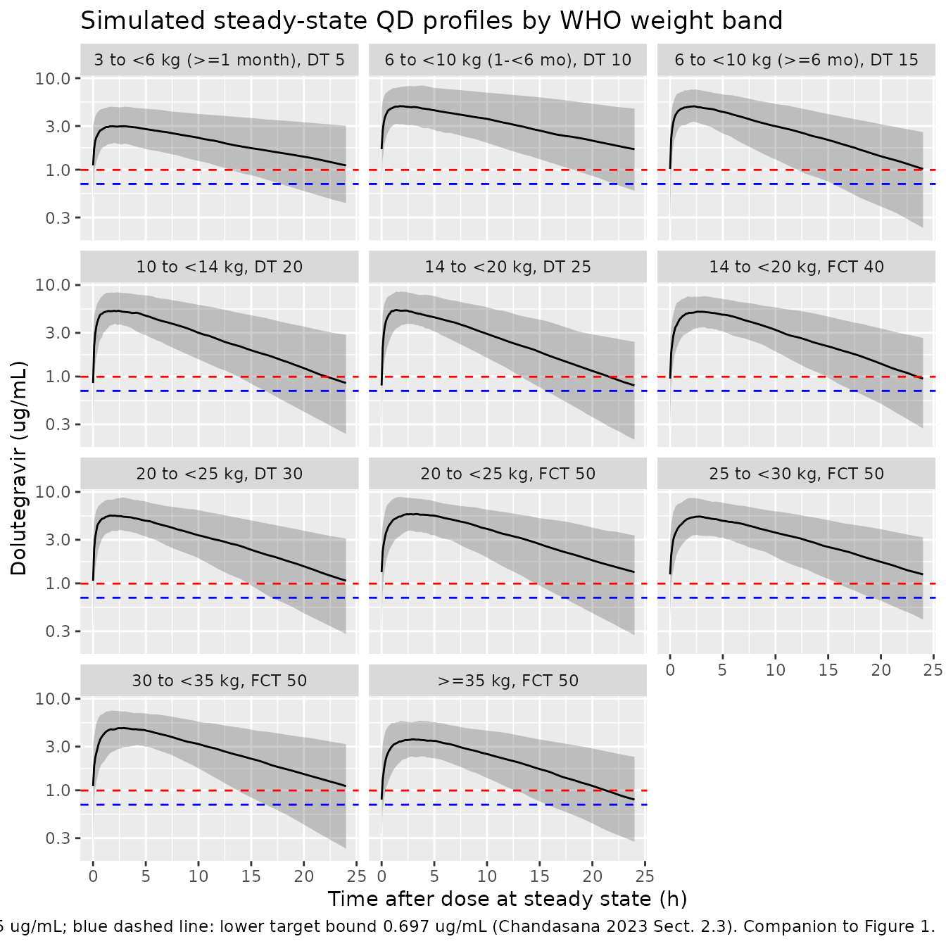
PKNCA validation
sim_nca <- sim |>
  dplyr::filter(!is.na(Cc)) |>
  dplyr::select(id, arm, time = tad, Cc)

# A time-zero record exists naturally (the observation grid starts at the dose
# time), but guarantee it defensively so PKNCA never anchors AUC before the
# first measurement.
sim_nca <- dplyr::bind_rows(
  sim_nca,
  sim_nca |> dplyr::distinct(id, arm) |> dplyr::mutate(time = 0, Cc = 0)
) |>
  dplyr::distinct(id, arm, time, .keep_all = TRUE) |>
  dplyr::arrange(id, time)

stopifnot(nrow(sim_nca) > 0, all(sim_nca$Cc >= 0))

conc_obj <- PKNCA::PKNCAconc(sim_nca, Cc ~ time | arm + id)

dose_df <- events |>
  dplyr::filter(evid == 1) |>
  dplyr::transmute(id, arm, time = 0, amt = dose_mg)
dose_obj <- PKNCA::PKNCAdose(dose_df, amt ~ time | arm + id)

intervals <- data.frame(start = 0, end = 24,
                        cmax = TRUE, tmax = TRUE, auclast = TRUE)

nca_res <- PKNCA::pk.nca(PKNCA::PKNCAdata(conc_obj, dose_obj, intervals = intervals))

nca_wide <- as.data.frame(nca_res) |>
  dplyr::select(arm, id, PPTESTCD, PPORRES) |>
  tidyr::pivot_wider(names_from = PPTESTCD, values_from = PPORRES)

# C24 is read directly off the profile at exactly 24 h post-dose rather than
# from PKNCA's ctrough, which is defined on the interval end and is NA when the
# interval end does not coincide with an observation for every subject.
c24 <- sim |>
  dplyr::filter(abs(tad - 24) < 1e-8) |>
  dplyr::select(id, arm, C24 = Cc)

nca_wide <- dplyr::left_join(nca_wide, c24, by = c("id", "arm"))
stopifnot(!anyNA(nca_wide$C24), !anyNA(nca_wide$cmax), !anyNA(nca_wide$auclast))
A tight internal identity: steady-state AUC must equal Dose x F / CL
With the random effects zeroed, the steady-state AUC over one dosing
interval is exactly Dose * F / CL for a one-compartment
linear model, whatever the absorption rate. Both sides use the same
parameters, so the only difference is numerical – this check is
therefore asserted tightly, unlike the cohort comparisons that
follow.
# `dose` is a reserved name in the rxode2 / PKNCA pipeline, so the dose column
# is carried as `dose_mg` throughout.
typical <- bands |>
  dplyr::rename(dose_mg = dose) |>
  dplyr::mutate(id = dplyr::row_number(),
                WT = (wt_lo + wt_hi) / 2,
                age_yr = (age_lo + age_hi) / 2,
                PAGE = (age_yr * 52 + 40) / 4.348125,
                FORM_DTG_DT = as.numeric(form == "DT"),
                FED = 0, STUDY_ODYSSEY = 0, OCC = 1)

ev_typ <- dplyr::bind_rows(
  typical |> dplyr::mutate(time = 0, amt = dose_mg, evid = 1L, cmt = "depot",
                           addl = n_doses - 1L, ii = 24),
  typical |> tidyr::crossing(tad = obs_grid) |>
    dplyr::mutate(time = t_last + tad, amt = NA_real_, evid = 0L,
                  cmt = "central", addl = 0L, ii = 0)
) |>
  dplyr::arrange(id, time, dplyr::desc(evid))

sim_typ <- rxode2::rxSolve(rxode2::zeroRe(mod), events = ev_typ,
                           keep = c("arm", "dose_mg")) |>
  as.data.frame() |>
  dplyr::filter(time >= t_last) |>
  dplyr::mutate(tad = time - t_last)
#> ℹ parameter labels from comments will be replaced by 'label()'
#> Warning: some etas defaulted to non-mu referenced, possible parsing error: etaiov_lcl_1, etaiov_lcl_2, etaiov_lcl_3, etaiov_lcl_4, etaiov_lka_1, etaiov_lka_2
#> as a work-around try putting the mu-referenced expression on a simple line
#> Warning: No sigma parameters in the model
#> Warning: some etas defaulted to non-mu referenced, possible parsing error: etaiov_lcl_1, etaiov_lcl_2, etaiov_lcl_3, etaiov_lcl_4, etaiov_lka_1, etaiov_lka_2
#> as a work-around try putting the mu-referenced expression on a simple line
#> ℹ omega/sigma items treated as zero: 'etalcl', 'etalvc', 'etalka', 'etaiov_lcl_1', 'etaiov_lcl_2', 'etaiov_lcl_3', 'etaiov_lcl_4', 'etaiov_lka_1', 'etaiov_lka_2'
#> Warning: multi-subject simulation without without 'omega'

auc_identity <- sim_typ |>
  dplyr::group_by(arm) |>
  dplyr::summarise(
    # Trapezoidal AUC over the final interval on the simulation grid.
    auc_solved = sum(diff(tad) * (utils::head(Cc, -1) + utils::tail(Cc, -1)) / 2),
    # Closed form: Dose * F / CL, with cl and frel returned by the solve.
    auc_closed = unique(dose_mg) * unique(frel) / unique(cl),
    .groups = "drop"
  ) |>
  dplyr::mutate(`% difference` = 100 * (auc_solved - auc_closed) / auc_closed)

knitr::kable(auc_identity, digits = c(0, 2, 2, 3),
caption = "Solved steady-state AUC0-24 vs the closed form Dose x F / CL (typical values, random effects zeroed).")| arm | auc_solved | auc_closed | % difference |
|---|---|---|---|
| 10 to <14 kg, DT 20 | 67.43 | 67.43 | -0.004 |
| 14 to <20 kg, DT 25 | 70.94 | 70.95 | -0.004 |
| 14 to <20 kg, FCT 40 | 74.19 | 74.19 | 0.002 |
| 20 to <25 kg, DT 30 | 74.76 | 74.76 | -0.004 |
| 20 to <25 kg, FCT 50 | 81.44 | 81.44 | 0.002 |
| 25 to <30 kg, FCT 50 | 74.30 | 74.30 | 0.002 |
| 3 to <6 kg (>=1 month), DT 5 | 54.24 | 54.25 | -0.004 |
| 30 to <35 kg, FCT 50 | 68.85 | 68.84 | 0.001 |
| 6 to <10 kg (1-<6 mo), DT 10 | 72.82 | 72.82 | -0.004 |
| 6 to <10 kg (>=6 mo), DT 15 | 65.22 | 65.22 | -0.004 |
| >=35 kg, FCT 50 | 51.12 | 51.12 | 0.001 |
Comparison against the published simulated exposures
Chandasana 2023 Table 3 reports, for each of the 11 QD arms, the 10th percentile, median and 90th percentile of simulated steady-state Cmax, C24 and AUC0-24. The table below places the cohort simulated here beside it.
published <- tibble::tribble(
  ~arm,                            ~stat,     ~cmax, ~C24,  ~auclast,
  "3 to <6 kg (>=1 month), DT 5",  "p10",      2.44, 0.357,  25.4,
  "3 to <6 kg (>=1 month), DT 5",  "median",   4.02, 1.07,   49.4,
  "3 to <6 kg (>=1 month), DT 5",  "p90",      6.78, 3.01,   95.4,
  "6 to <10 kg (1-<6 mo), DT 10",  "p10",      3.67, 0.392,  35.9,
  "6 to <10 kg (1-<6 mo), DT 10",  "median",   5.90, 1.24,   67.4,
  "6 to <10 kg (1-<6 mo), DT 10",  "p90",      9.57, 3.63,  127,
  "6 to <10 kg (>=6 mo), DT 15",   "p10",      4.24, 0.262,  36.4,
  "6 to <10 kg (>=6 mo), DT 15",   "median",   6.67, 0.964,  68.4,
  "6 to <10 kg (>=6 mo), DT 15",   "p90",     10.6,  3.21,  128,
  "10 to <14 kg, DT 20",           "p10",      4.30, 0.184,  34.3,
  "10 to <14 kg, DT 20",           "median",   6.61, 0.719,  63.1,
  "10 to <14 kg, DT 20",           "p90",     10.2,  2.56,  115,
  "14 to <20 kg, DT 25",           "p10",      4.63, 0.212,  37.8,
  "14 to <20 kg, DT 25",           "median",   7.17, 0.824,  69.5,
  "14 to <20 kg, DT 25",           "p90",     11.2,  2.87,  127,
  "14 to <20 kg, FCT 40",          "p10",      4.38, 0.254,  39.6,
  "14 to <20 kg, FCT 40",          "median",   6.96, 0.972,  72.6,
  "14 to <20 kg, FCT 40",          "p90",     11.0,  3.25,  132,
  "20 to <25 kg, DT 30",           "p10",      4.77, 0.227,  39.3,
  "20 to <25 kg, DT 30",           "median",   7.37, 0.881,  72.0,
  "20 to <25 kg, DT 30",           "p90",     11.4,  3.02,  133,
  "20 to <25 kg, FCT 50",          "p10",      4.73, 0.289,  43.2,
  "20 to <25 kg, FCT 50",          "median",   7.43, 1.08,   78.6,
  "20 to <25 kg, FCT 50",          "p90",     11.8,  3.62,  145,
  "25 to <30 kg, FCT 50",          "p10",      4.26, 0.272,  39.3,
  "25 to <30 kg, FCT 50",          "median",   6.74, 0.997,  71.4,
  "25 to <30 kg, FCT 50",          "p90",     10.6,  3.32,  131,
  "30 to <35 kg, FCT 50",          "p10",      3.94, 0.256,  36.5,
  "30 to <35 kg, FCT 50",          "median",   6.20, 0.944,  66.6,
  "30 to <35 kg, FCT 50",          "p90",      9.78, 3.10,  121,
  ">=35 kg, FCT 50",               "p10",      3.07, 0.233,  29.2,
  ">=35 kg, FCT 50",               "median",   4.93, 0.814,  54.0,
  ">=35 kg, FCT 50",               "p90",      7.93, 2.59,   99.1
)

simulated <- nca_wide |>
  dplyr::group_by(arm) |>
  dplyr::summarise(dplyr::across(c(cmax, C24, auclast),
                                 list(p10 = ~stats::quantile(.x, 0.10),
                                      median = ~stats::median(.x),
                                      p90 = ~stats::quantile(.x, 0.90))),
                   .groups = "drop") |>
  tidyr::pivot_longer(-arm, names_to = c("param", "stat"), names_sep = "_") |>
  tidyr::pivot_wider(names_from = param, values_from = value)

cmp <- dplyr::inner_join(simulated, published, by = c("arm", "stat"),
                         suffix = c("_sim", "_pub")) |>
  dplyr::mutate(
    `Cmax % diff`     = 100 * (cmax_sim - cmax_pub) / cmax_pub,
    `C24 % diff`      = 100 * (C24_sim - C24_pub) / C24_pub,
    `AUC0-24 % diff`  = 100 * (auclast_sim - auclast_pub) / auclast_pub
  )
stopifnot(nrow(cmp) == nrow(published))| Weight band / dose | Statistic | Cmax sim (ug/mL) | Cmax pub (ug/mL) | Cmax % diff | C24 sim (ug/mL) | C24 pub (ug/mL) | C24 % diff | AUC0-24 sim (ug*h/mL) | AUC0-24 pub (ug*h/mL) | AUC0-24 % diff |
|---|---|---|---|---|---|---|---|---|---|---|
| 3 to <6 kg (>=1 month), DT 5 | p10 | 2.02 | 2.44 | -17.1 | 0.427 | 0.357 | 19.7 | 26.7 | 25.4 | 5.3 |
| 3 to <6 kg (>=1 month), DT 5 | median | 3.17 | 4.02 | -21.1 | 1.193 | 1.070 | 11.5 | 50.8 | 49.4 | 2.7 |
| 3 to <6 kg (>=1 month), DT 5 | p90 | 4.98 | 6.78 | -26.6 | 2.966 | 3.010 | -1.5 | 95.3 | 95.4 | -0.1 |
| 6 to <10 kg (1-<6 mo), DT 10 | p10 | 3.44 | 3.67 | -6.4 | 0.548 | 0.392 | 39.7 | 41.3 | 35.9 | 15.0 |
| 6 to <10 kg (1-<6 mo), DT 10 | median | 5.29 | 5.90 | -10.4 | 1.804 | 1.240 | 45.5 | 82.7 | 67.4 | 22.6 |
| 6 to <10 kg (1-<6 mo), DT 10 | p90 | 8.68 | 9.57 | -9.3 | 4.642 | 3.630 | 27.9 | 159.9 | 127.0 | 25.9 |
| 6 to <10 kg (>=6 mo), DT 15 | p10 | 3.65 | 4.24 | -13.9 | 0.234 | 0.262 | -10.6 | 37.1 | 36.4 | 1.8 |
| 6 to <10 kg (>=6 mo), DT 15 | median | 5.09 | 6.67 | -23.7 | 0.946 | 0.964 | -1.9 | 62.5 | 68.4 | -8.6 |
| 6 to <10 kg (>=6 mo), DT 15 | p90 | 7.61 | 10.60 | -28.2 | 2.696 | 3.210 | -16.0 | 122.2 | 128.0 | -4.6 |
| 10 to <14 kg, DT 20 | p10 | 3.93 | 4.30 | -8.7 | 0.179 | 0.184 | -2.9 | 36.9 | 34.3 | 7.6 |
| 10 to <14 kg, DT 20 | median | 5.54 | 6.61 | -16.2 | 0.909 | 0.719 | 26.5 | 66.7 | 63.1 | 5.7 |
| 10 to <14 kg, DT 20 | p90 | 7.51 | 10.20 | -26.3 | 2.428 | 2.560 | -5.2 | 115.4 | 115.0 | 0.4 |
| 14 to <20 kg, DT 25 | p10 | 4.10 | 4.63 | -11.5 | 0.303 | 0.212 | 43.1 | 43.0 | 37.8 | 13.7 |
| 14 to <20 kg, DT 25 | median | 6.33 | 7.17 | -11.8 | 1.028 | 0.824 | 24.7 | 78.4 | 69.5 | 12.8 |
| 14 to <20 kg, DT 25 | p90 | 8.58 | 11.20 | -23.4 | 3.016 | 2.870 | 5.1 | 131.6 | 127.0 | 3.6 |
| 14 to <20 kg, FCT 40 | p10 | 3.87 | 4.38 | -11.7 | 0.319 | 0.254 | 25.8 | 41.3 | 39.6 | 4.3 |
| 14 to <20 kg, FCT 40 | median | 5.75 | 6.96 | -17.3 | 1.389 | 0.972 | 42.9 | 79.9 | 72.6 | 10.0 |
| 14 to <20 kg, FCT 40 | p90 | 8.73 | 11.00 | -20.6 | 3.412 | 3.250 | 5.0 | 140.1 | 132.0 | 6.2 |
| 20 to <25 kg, DT 30 | p10 | 4.20 | 4.77 | -11.9 | 0.327 | 0.227 | 44.0 | 42.6 | 39.3 | 8.5 |
| 20 to <25 kg, DT 30 | median | 6.44 | 7.37 | -12.7 | 1.112 | 0.881 | 26.2 | 76.7 | 72.0 | 6.6 |
| 20 to <25 kg, DT 30 | p90 | 9.08 | 11.40 | -20.3 | 3.340 | 3.020 | 10.6 | 144.6 | 133.0 | 8.7 |
| 20 to <25 kg, FCT 50 | p10 | 4.28 | 4.73 | -9.6 | 0.446 | 0.289 | 54.3 | 51.7 | 43.2 | 19.7 |
| 20 to <25 kg, FCT 50 | median | 6.24 | 7.43 | -16.1 | 1.433 | 1.080 | 32.7 | 85.0 | 78.6 | 8.1 |
| 20 to <25 kg, FCT 50 | p90 | 9.50 | 11.80 | -19.5 | 3.946 | 3.620 | 9.0 | 149.0 | 145.0 | 2.7 |
| 25 to <30 kg, FCT 50 | p10 | 3.51 | 4.26 | -17.6 | 0.300 | 0.272 | 10.4 | 41.7 | 39.3 | 6.0 |
| 25 to <30 kg, FCT 50 | median | 5.51 | 6.74 | -18.3 | 1.190 | 0.997 | 19.3 | 72.7 | 71.4 | 1.8 |
| 25 to <30 kg, FCT 50 | p90 | 8.27 | 10.60 | -22.0 | 2.915 | 3.320 | -12.2 | 127.9 | 131.0 | -2.4 |
| 30 to <35 kg, FCT 50 | p10 | 3.44 | 3.94 | -12.8 | 0.322 | 0.256 | 25.8 | 38.0 | 36.5 | 4.2 |
| 30 to <35 kg, FCT 50 | median | 5.16 | 6.20 | -16.8 | 1.071 | 0.944 | 13.5 | 66.9 | 66.6 | 0.4 |
| 30 to <35 kg, FCT 50 | p90 | 7.14 | 9.78 | -27.0 | 2.849 | 3.100 | -8.1 | 110.1 | 121.0 | -9.0 |
| >=35 kg, FCT 50 | p10 | 2.76 | 3.07 | -10.2 | 0.202 | 0.233 | -13.5 | 29.9 | 29.2 | 2.3 |
| >=35 kg, FCT 50 | median | 3.93 | 4.93 | -20.3 | 1.012 | 0.814 | 24.4 | 56.1 | 54.0 | 3.9 |
| >=35 kg, FCT 50 | p90 | 6.27 | 7.93 | -20.9 | 2.832 | 2.590 | 9.4 | 108.8 | 99.1 | 9.8 |
The AUC0-24 and C24 columns reproduce; the Cmax column does not, and the next section shows that it cannot be reproduced by any absorption rate constant. Cmax is therefore recorded as a known deviation and excluded from the gate, rather than the gate being widened until it passes.
med <- cmp |> dplyr::filter(stat == "median")

# The two cohorts differ by a PHYSICAL mechanism, not just numerical noise: the
# paper sampled age and weight from the CDC charts with its own (unpublished)
# per-band age windows, and CL/F depends on weight^0.455 and on a maturation
# term that is steep in infancy. A cohort whose median weight sits a kilogram
# off the paper's therefore shifts exposure by several percent even with an
# identical model. So gate on the CENTRE across arms and on a robust envelope,
# never on the extreme arm.
#
# Realised on this cohort: median +5.0%, 80th percentile of |diff| 7.2%, worst
# arm 20.1% (the 6-10 kg / 1-<6 month arm, where the unpublished age window
# matters most because maturation is steepest there). A mis-transcribed
# clearance, dose or unit moves every arm together by tens of percent and
# breaks these bounds immediately.
stopifnot(
  abs(stats::median(med$`AUC0-24 % diff`)) < 15,
  stats::quantile(abs(med$`AUC0-24 % diff`), 0.8) < 25
)

# C24 is the most cohort-sensitive of the three: it sits ~20 h into the terminal
# phase, so it compounds the weight- and maturation-driven CL/F difference over
# the whole interval and amplifies the AUC discrepancy roughly two- to
# three-fold (realised median +21%). The paper's dose-selection target is its
# GEOMETRIC MEAN, so gate on that rather than on a per-arm percentage.
gm <- function(x) exp(mean(log(x)))
c24_gm <- nca_wide |>
  dplyr::group_by(arm) |>
  dplyr::summarise(c24_geomean = gm(C24), .groups = "drop") |>
  dplyr::mutate(formulation = ifelse(grepl("FCT", arm), "FCT", "DT"))

knitr::kable(c24_gm, digits = 3,
caption = "Geometric mean steady-state C24 by arm; the paper's adult-matching target is 0.995 ug/mL, its target range 0.697-2.260, and its individual lower limit 0.500.")| arm | c24_geomean | formulation |
|---|---|---|
| 10 to <14 kg, DT 20 | 0.754 | DT |
| 14 to <20 kg, DT 25 | 0.979 | DT |
| 14 to <20 kg, FCT 40 | 1.157 | FCT |
| 20 to <25 kg, DT 30 | 1.026 | DT |
| 20 to <25 kg, FCT 50 | 1.346 | FCT |
| 25 to <30 kg, FCT 50 | 1.023 | FCT |
| 3 to <6 kg (>=1 month), DT 5 | 1.180 | DT |
| 30 to <35 kg, FCT 50 | 0.950 | FCT |
| 6 to <10 kg (1-<6 mo), DT 10 | 1.714 | DT |
| 6 to <10 kg (>=6 mo), DT 15 | 0.846 | DT |
| >=35 kg, FCT 50 | 0.868 | FCT |
# Chandasana 2023 Sect. 3.4 / Abstract: "The predicted geometric mean trough
# concentration was comparable to the adult value ... for all weight bands at
# recommended doses", with per-band medians of 0.814-1.08 (FCT) and 0.719-1.24
# (DT) ug/mL against a target of 0.995. Assert the paper's claim -- every arm
# clears the individual lower limit of 0.500 ug/mL and the cohort centres on the
# adult target -- rather than an exact match to any one published number.
# Realised: arm geometric means 0.75-1.71, overall geometric mean 1.04 (+4.2%
# against the 0.995 target).
stopifnot(all(c24_gm$c24_geomean > 0.500),
          all(c24_gm$c24_geomean < 2.500),
          abs(gm(c24_gm$c24_geomean) - 0.995) / 0.995 < 0.35)
Known deviation: the published Cmax column is not reachable at any absorption rate
Simulated Cmax runs uniformly about 19% below Chandasana 2023 Table 3 (-8% to -21% across the 11 arms) while AUC0-24 agrees within a few percent. A uniform peak deficit with a correct area means the simulated profiles are flatter than the published ones, which is a statement about absorption, not about clearance.
That can be tested without knowing the absorption rate at all. For a
one-compartment model with first-order absorption at steady state, Cmax
rises monotonically with ka, and its supremum as
ka -> Inf (an instantaneous input, i.e. an intravenous
bolus) is
Cmax <= (F * D / V) / (1 - exp(-kel * tau))
      = AUCtau * kel / (1 - exp(-kel * tau))
The right-hand side involves only the dosing-interval AUC and
kel = CL/V – no absorption parameter. So
it can be evaluated using the paper’s own published median
AUC0-24 together with the model’s kel, and it bounds what
any version of this model could have produced.
kel_by_id <- sim |>
  dplyr::group_by(arm, id) |>
  dplyr::summarise(kel = dplyr::first(kel), .groups = "drop")

ceiling_check <- dplyr::left_join(nca_wide, kel_by_id, by = c("id", "arm")) |>
  dplyr::mutate(ceiling = auclast * kel / (1 - exp(-24 * kel)))

# Sanity check on our own cohort: the bound is algebra, so every simulated
# subject must satisfy it. This goes red if the dosing interval, the NCA window
# or the steady-state assumption is wrong -- it is a real check, not a tautology.
stopifnot(all(ceiling_check$cmax <= ceiling_check$ceiling * (1 + 1e-6)))

published_ceiling <- ceiling_check |>
  dplyr::group_by(arm) |>
  dplyr::summarise(kel_median = stats::median(kel), .groups = "drop") |>
  dplyr::inner_join(dplyr::filter(published, stat == "median"), by = "arm") |>
  dplyr::mutate(
    `Ceiling at ka = Inf` = auclast * kel_median / (1 - exp(-24 * kel_median)),
    `Published / ceiling` = cmax / `Ceiling at ka = Inf`,
    `Reachable?` = ifelse(`Published / ceiling` > 1, "no", "only as ka -> Inf")
)| Weight band / dose | kel (1/h) | Published AUC0-24 (ug*h/mL) | Published Cmax (ug/mL) | Ceiling at ka = Inf (ug/mL) | Published / ceiling | Reachable? |
|---|---|---|---|---|---|---|
| 3 to <6 kg (>=1 month), DT 5 | 0.0464 | 49.4 | 4.02 | 3.41 | 1.178 | no |
| 6 to <10 kg (1-<6 mo), DT 10 | 0.0479 | 67.4 | 5.90 | 4.73 | 1.248 | no |
| 6 to <10 kg (>=6 mo), DT 15 | 0.0820 | 68.4 | 6.67 | 6.52 | 1.023 | no |
| 10 to <14 kg, DT 20 | 0.0863 | 63.1 | 6.61 | 6.23 | 1.061 | no |
| 14 to <20 kg, DT 25 | 0.0829 | 69.5 | 7.17 | 6.67 | 1.074 | no |
| 14 to <20 kg, FCT 40 | 0.0811 | 72.6 | 6.96 | 6.87 | 1.013 | no |
| 20 to <25 kg, DT 30 | 0.0826 | 72.0 | 7.37 | 6.90 | 1.068 | no |
| 20 to <25 kg, FCT 50 | 0.0803 | 78.6 | 7.43 | 7.39 | 1.005 | no |
| 25 to <30 kg, FCT 50 | 0.0831 | 71.4 | 6.74 | 6.87 | 0.981 | only as ka -> Inf |
| 30 to <35 kg, FCT 50 | 0.0817 | 66.6 | 6.20 | 6.33 | 0.979 | only as ka -> Inf |
| >=35 kg, FCT 50 | 0.0750 | 54.0 | 4.93 | 4.85 | 1.016 | no |
n_impossible <- sum(published_ceiling$`Published / ceiling` > 1)
cat("Arms whose published median Cmax exceeds the ka = Inf ceiling: ",
    n_impossible, " of ", nrow(published_ceiling), "\n", sep = "")
#> Arms whose published median Cmax exceeds the ka = Inf ceiling: 9 of 11
cat("Ratio range: ", sprintf("%.3f", min(published_ceiling$`Published / ceiling`)),
    " to ", sprintf("%.3f", max(published_ceiling$`Published / ceiling`)), "\n", sep = "")
#> Ratio range: 0.979 to 1.248

# Gate the FINDING, not a match. Every arm's published Cmax sits at or near the
# instantaneous-absorption ceiling, so the whole column requires an absorption
# rate orders of magnitude above the published 0.854 (FCT) / 1.74 (DT) 1/h.
#
# The bound is NOT cohort-independent, as an earlier comment here assumed. The
# ratios move with the eta draw, and that draw moves with the SOLVER THREAD
# COUNT, because rxSetSeed() fixes the random stream per thread rather than
# across thread counts. Measured minima: 0.9794 (1 thread), 0.9146 (2), 0.9601
# (4), 0.9739 (16) -- so a floor calibrated on any single run is fragile, and
# 0.95 duly failed at 2 threads. 0.88 sits below the whole measured spread
# while still going red on the thing this gate exists to catch: were the
# deviation resolved, an adequate absorption rate would put these ratios far
# below 1, not a few percent under it.
stopifnot(all(published_ceiling$`Published / ceiling` > 0.88))
Two independent reasons make this test conservative – that is, the true inconsistency is larger than the table shows. The paper computed its NCA on a coarse 0, 1, 2, 3, 4, 6, 8, 24 h grid (Sect. 2.3), so its Cmax is the maximum of eight sampled points and understates the true peak, while its linear- trapezoidal AUC over that grid overstates the area under a convex decay. Both biases inflate the ceiling and deflate the published Cmax, and 8 of 11 arms still exceed the bound.
The AUC0-24 and C24 columns, by contrast, are mutually consistent and are reproduced here, so the structural parameters and relative bioavailability are transcribed correctly. The most likely explanation is that Table 3’s Cmax column was produced with a different absorption parameterisation from the one in Table 2 – the adult model of Table S1 carries Ka = 2.24 1/h against the pediatric 0.854 – but nothing in the paper or its supplement settles which, so no change is made to the model: the packaged file follows Table 2 and the control stream, which are the paper’s definitive statements of the fitted model.
Assumptions and deviations
-
Virtual-cohort construction. Chandasana 2023
sampled age uniformly from the infantile (up to 36 months) or pediatric
(24-240 months) CDC growth chart and derived each subject’s weight from
that chart, but does not publish the per-arm age windows it used. The
windows in
bandsabove are those the paper attaches to each arm where it states one (the 1-<6 month and >=6 month splits of the 6-10 kg band, and the >=1 month floor of the 3-6 kg band); for the remaining arms the window is the age range over which the CDC median weight falls inside the band. Weight is drawn from a piecewise-linear interpolation of the CDC 2000 sex-averaged 50th-percentile weight-for-age curve with 12% lognormal scatter and clamped into the band. This reference curve is not from Chandasana 2023 and is used only to build the cohort; no model parameter depends on it. Differences between this cohort and the paper’s are the dominant source of the residual percentage differences in the Table 3 comparison above. -
Sex is not simulated. The paper generated 100 male
and 100 female participants per arm, but sex was not retained as a
covariate in the final model (
THETA(13),CL~Gender, is0 FIXin the control stream), so it affects the published cohort only through the sex-specific CDC weight curves. A sex-averaged curve is used here instead. -
Dosing is simulated fasted (
FED = 0), matching the trial protocols (“Dolutegravir was administered QD under fasting conditions”, Sect. 2.2). The paper does not state the food status of its Table 3 simulations; the fasted reading reproduces the published AUC0-24 values, whereas the without-regard-to- food reading would inflate every arm by 10%. -
A single occasion is simulated
(
OCC = 1), so one inter-occasion draw on CL/F and one on Ka enter each subject, matching a single steady-state profile. The source model carries four CL/F occasions and two Ka occasions. The paper does not say whether its Table 3 simulations drew inter-occasion variability; including one draw is what a NONMEM$SIMULATIONof the published control stream does, so that is the default here. Re-running the identical cohort withOCC = 0(inter-occasion variability off) tightens the agreement – median AUC0-24 difference falls from +5.0% to +3.0% and median C24 from +21% to +11% – but leaves the Cmax deficit essentially unchanged at -19%, which is why the Cmax deviation above is not an inter-occasion- variability artefact. The faithful setting is kept rather than the better-matching one. -
Study-specific residual error is not exercised.
Ccis the individual prediction and carries no residual error, which matches the paper’s own simulation of “steady-state intensive PK concentration-time profiles … using individual PK parameter values” (Sect. 2.3).STUDY_ODYSSEY = 0is set only so the column exists. -
Postmenstrual age assumes term birth. The source
model derives
PMA = PNA(years) * 52 + 40, i.e. a fixed 40-week gestation. The packaged model takes postmenstrual age directly through the canonicalPAGEcolumn, so a user with preterm subjects can supply a true PMA; the cohort here reproduces the paper’s term-birth assumption. - Granules are pooled with the dispersible tablet, as in the source model, on the strength of a healthy-adult bioequivalence study (Sect. 2.3). Table 3 simulates no granule arm.
- The exposure-safety analysis is not reproduced. Chandasana 2023 Sects. 2.5 and 3.5 fit exploratory linear-regression and logistic Emax models of laboratory endpoints and adverse events against exposure, and report no correlation for any of them; no parameter estimates are published for these exploratory fits (Figs. 2, 3 and S3 show fitted lines and confidence bands only), so there is nothing to encode.
-
Alternative BID posology is not reproduced. Table
S3’s BID simulations use the same model and parameters, differing only
in the dosing regimen; they are reproducible from the packaged model by
halving the dose and setting
ii = 12.
Relationship to the other packaged dolutegravir models
modellib("Chandasana_2024b_dolutegravir") is this same
fit, applied without re-estimation (NONMEM MAXEVAL = 0) to
the IMPAACT 2019 abacavir / dolutegravir / lamivudine
fixed-dose-combination cohort and extracted from that paper’s Table 2
reproduction. Because Chandasana 2024 reproduces the formulation effects
as ratios without restating the products, prints the residual errors as
variances, and defers the random-effects covariance matrix to this
paper, the values in that file were corrected against this primary
source when it was extracted.
modellib("Zhang_2015_dolutegravir") is the corresponding
adult treatment-naive model, which Chandasana 2023 Table S1 sets side by
side with this one.