Benzylpenicillin in horses, PK/PD cutoffs (Lallemand 2023) • nlmixr2lib

Model and source

Citation: Lallemand EA, Bousquet-Melou A, Chapuis L, Davis J, Ferran AA, Kukanich B, Kuroda T, Lacroix MZ, Minamijima Y, Olsen L, Pelligand L, Portugal FR, Roques BB, Santschi EM, Wilson KE, Toutain P-L. Pharmacokinetic-pharmacodynamic cutoff values for benzylpenicillin in horses to support the establishment of clinical breakpoints for benzylpenicillin antimicrobial susceptibility testing in horses. Front Microbiol. 2023;14:1282949. doi:10.3389/fmicb.2023.1282949
Article: Front Microbiol. 2023;14:1282949
Supplement (open access, Data Sheet 1): https://www.frontiersin.org/articles/10.3389/fmicb.2023.1282949/full#supplementary-material

The supplement is load-bearing for this extraction. Supplementary Data 2 contains the complete Phoenix NLME control stream for the final model, Supplementary Table S7 lists every typical value (the main-text Table 6 is explicitly only “a selection”), Supplementary Table S8 lists the model-derived secondary parameters used as validation targets below, and Supplementary Tables S13-S21 hold the Monte Carlo PK/PD cutoff results this vignette reproduces.

Population

The model is an international meta-analysis assembled for the VetCAST clinical-breakpoint project. Raw data from 40 horses provided 63 rich concentration-time profiles and 1,022 benzylpenicillin (BP) plasma concentrations, pooled from five datasets: France (n = 6), Sweden (n = 15), Japan (n = 6), USA1 (n = 7) and USA2 (n = 6). Horses weighed 308-592 kg and were 4-24 years old (age unreported for 2 horses); 20 were mares/females, 15 geldings, 4 stallions and 1 unrecorded (Supplementary Table S3). Breeds were Standardbred trotters (Sweden), Thoroughbreds (Japan, USA2), Quarter Horses / Paint / Thoroughbred (USA1), French Trotters, Arabian and Spanish half-bloods and a Saddlebred (France), plus one mixed pony. All horses were healthy; none had a clinical infection.

Designs were deliberately unbalanced: no IV data in Japan, IV data only in USA2, and limits of quantification differing by site (5.5 ng/mL Sweden, 10 ng/mL France and USA1, 30 ng/mL Japan, 40 ng/mL USA2). BLOQ values (<5% of measurements) were discarded. All concentrations were measured by LC-MS/MS.

Because the objective was the most generic PK/PD cutoff possible, no biological covariate (body weight, age, sex, breed) was carried into the model. The single covariate is 'source of dataset', retained on plasma clearance so that the bioavailability of each formulation could be estimated against the clearance of the horses that actually received it (Lallemand 2023 Section 2.2).

str(meta$population, max.level = 1)
#> List of 14
#>  $ species       : chr "horse (Equus caballus); Standardbred trotters (Sweden), Thoroughbreds (Japan, USA2), Quarter Horses / Quarter H"| __truncated__
#>  $ n_subjects    : int 40
#>  $ n_studies     : int 5
#>  $ n_profiles    : int 63
#>  $ n_observations: int 1022
#>  $ age_range     : chr "4-24 years (Supplementary Table S3; age not reported for 2 of the 40 horses)"
#>  $ weight_range  : chr "308-592 kg (Supplementary Table S3)"
#>  $ sex_female_pct: num 50
#>  $ sex_notes     : chr "20 mares/females, 15 geldings, 4 stallions/males, 1 horse with sex not reported (Supplementary Table S3)"
#>  $ disease_state : chr "healthy adult horses enrolled in experimental pharmacokinetic trials; no clinical infection"
#>  $ dose_range    : chr "5.617-25.11 mg/kg expressed as benzylpenicillin base (Supplementary Table S2); the reference regimen throughout"| __truncated__
#>  $ regions       : chr "France, Sweden, Japan, United States (two independent US datasets, USA1 and USA2)"
#>  $ formulations  : chr "IV sodium BP (France, Sweden), IV potassium BP (USA1, USA2), IM procaine BP (France Depocilline, Sweden Penovet"| __truncated__
#>  $ notes         : chr "Meta-analysis assembled for the VetCAST clinical-breakpoint project. The French data were generated specificall"| __truncated__

Model structure

The authors fitted one simultaneous model to all IV and IM data, sharing a single set of disposition parameters across every route and formulation. The packaged model reproduces that structure with seven absorption depots feeding one three-compartment disposition system (Lallemand 2023 Figure 4):

Depot	Modality	Absorption structure
(none - dose `central`)	IV sodium or potassium BP	bolus or infusion
`depot1`	IM sodium BP (Geepenil)	sequential: rapid `ka` until `tlag`, then slow `ka2`
`depot2`	IM procaine BP, 4 single-ingredient products	single `ka`, dataset covariate on `ka` and on logit `F`
`depot3`	procaine BP fraction of Duplocilline	single `ka` (parallel with `depot4`)
`depot4`	benzathine BP fraction of Duplocilline	single `ka` (parallel with `depot3`)
`depot5`, `depot6`, `depot7`	IM penethamate, injection sites 1-3	sequential per site: rapid then slow `ka`, each with its own delay

Because the assay measures a single analyte (BP in plasma), all seven depots feed the same central compartment. This is exactly equivalent to the published Phoenix code, which summed the contributions of the Duplocilline components (CBenza1 + CBenza2) and of the three penethamate sites (CPenethamate1 + CPenethamate2 + CPenethamate3) before comparing with the observations.

The two sequential-absorption structures are implemented with tad(<depot>), the time since that depot’s most recent dose. Supplementary Data 2 achieved the same effect with hard-coded sequence{} blocks that had to enumerate every dose time; tad() restores the generality, so the switch fires correctly for any regimen the user simulates.

mod <- rxode2::rxode2(mod_fun)
cat("ODE states:", paste(mod$state, collapse = ", "), "\n")
#> ODE states: depot1, depot2, depot3, depot4, depot5, depot6, depot7, central, peripheral1, peripheral2, auc_free, t_above_mic

Source trace

Every ini() entry in inst/modeldb/specificDrugs/Lallemand_2023_benzylpenicillin_horse.R carries an in-file comment pointing at its source. The table collects them for review. “SD2” is Supplementary Data 2 (the Phoenix control stream); “S7”/“S8” are Supplementary Tables S7/S8.

Parameter	Value	Source location
`lvc` (Vc)	106.184 mL/kg	SD2 `fixef(tvV(freeze))`; Table 4, S7 (106)
`lvp` (V2)	46.295 mL/kg	SD2 `fixef(tvV2(freeze))`; Table 4 (46.3)
`lvp2` (V3)	50.430 mL/kg	SD2 `fixef(tvV3(freeze))`; Table 4 (50.4)
`lcl` (CL, France)	480.899 mL/kg/h	SD2 `fixef(tvCl(freeze))`; Table 4, S7 (481)
`lq` (CL2)	125.961 mL/kg/h	SD2 `fixef(tvCl2(freeze))`; Table 4 (126)
`lq2` (CL3)	24.982 mL/kg/h	SD2 `fixef(tvCl3(freeze))`; Table 4 (25.0)
`e_study_sweden_iv_cl`	-0.683254	Table 4 `dCldSource_of_data1`; S7 `dCldNationcode1`
`e_study_usa1_cl`	-0.125766	Table 4 `dCldSource_of_data2`; S7 `dCldNationcode2`
`e_study_usa2_cl`	-0.136097	Table 4 `dCldSource_of_data3`; S7 `dCldNationcode4`
`e_study_japan_cl`	-0.156692	SD2 `fixef(dCldNationcode3)`; S7 (-0.1567)
`e_study_sweden_im_cl`	-0.314631	SD2 `fixef(dCldNationcode11)`; S7 (-0.3146)
`lka_im_na`, `lka2_im_na`	1.02419, 0.248124 /h	SD2 `tvKa1PeniNa`, `tvKa2PeniNa`; Table 6, S7
`ltlag_im_na`	0.470980 h	SD2 `tvtlagPeni`; Table 6, S7 (0.471)
`lfdepot_im_na`	0.891329	SD2 `tvFPeniNa`; Table 6, S7 (89.1%)
`lka_proc`	0.0465948 /h	SD2 `tvKaPROC`; S7 (0.0466)
`e_study_*_ka_proc`	0.03901, -2.37156, -0.00427	SD2 `dKadNationcode11/2/3`; S7
`logitfdepot_proc`	7.83103	SD2 `tvFPROC`; S7 (7.8310)
`e_study_*_fdepot_proc`	-0.00178, 0.05172, 0.42268	SD2 `dFNationcode11/2/3`; S7
`lka_duplo_pro`, `logitfdepot_duplo_pro`	0.0827110 /h, 1.53153	SD2 `tvKaBenza1`, `tvFBenza1`; Table 6, S7
`lka_duplo_benza`, `logitfdepot_duplo_benza`	0.00935420 /h, 10.9422	SD2 `tvKaBenza2`, `tvFBenza2`; Table 6, S7
`lka_peneth1/2/3`	0.0350071, 0.0223224, 0.0151705 /h	SD2 `tvKaPenethamate1/2/3`; S7
`lka2_peneth1/2/3`	0.0141804, 0.108334, 0.00162234 /h	SD2 `tvKaPenethamate_slow1/2/3`; S7
`ltlag_peneth1/2/3`	70.648, 27.217, 42.349 h	SD2 `tvtlag1/2/3`; S7 (70.6, 27.2, 42.3)
`logitfdepot_peneth`	0.788808	SD2 `tvFPenethamate`; S7 (68.8%)
`fu`	0.4 (fixed)	Section 2.3; binding 62.8% in Swedish horses (Olsen 2013)
`mic`	0.25 mg/L (fixed, adjustable)	Section 2.3; the paper’s concluded PK/PD cutoff
disposition OMEGA block (frozen)	6x6	SD2 `ranef(block(nV, nCl, nV2, nV3, nCl2, nCl3)(freeze))`
sodium BP OMEGA block	4x4	SD2 `ranef(block(nFPeniNa, ntlagPeni, nKa1PeniNA, nKa2PeniNA))`
Duplocilline OMEGA block	4x4	SD2 `ranef(block(nKaBenza1, nKaBenza2, nFBenza1, nFBenza2))`
procaine OMEGA block	2x2	SD2 `ranef(block(nKaPROC, nFPROC))`
penethamate OMEGA blocks (frozen)	3 x 2x2 + 1x1	SD2 `ranef(block(nKaPenethamate<i>, nKaPenethamate_slow<i>)(freeze))`
`propSd`	0.283453	SD2 `fixef(tvCMultStdev)`; Table 6, S7 (0.283)
`addSd_iv/_na_im/_duplo/_proc/_peneth`	0.007928, 0.162677, 0.006537, 0.004579, 0.008068 ug/mL	SD2 `error(CEps*)`; S7 `stdev0`-`stdev4`
Duplocilline composition split	5.96376 / 12.4 as procaine BP	Supplementary Table S2
ODE system (3-cmt, clearance form)	n/a	SD2 `deriv(A1... = -ClC1 - Cl2(C1-C2) - Cl3*(C1-C3))`
ilogit bioavailability transform	n/a	Equation 3; SD2 `stparm(F... = ilogit(...))`
Residual model (add + prop)	n/a	Section 2.2; SD2 `observe(CObs = C + CEpssqrt(1 + C^2(CMultStdev/sigma())^2))`

Verification of the published secondary parameters

The strongest available check is that the packaged parameters reproduce Lallemand 2023 Supplementary Table S8 (secondary parameters of the full model) and the nation-specific clearances of Table 6. These are deterministic functions of the ini() values, so the comparison is exact and every assertion below is strict.

th <- mod$theta
g <- function(n) unname(th[[n]])
ilogit <- function(x) 1 / (1 + exp(-x))

vc <- exp(g("lvc")); vp <- exp(g("lvp")); vp2 <- exp(g("lvp2"))
cl <- exp(g("lcl")); q <- exp(g("lq")); q2 <- exp(g("lq2"))

kel <- cl / vc; k12 <- q / vc; k13 <- q2 / vc; k21 <- q / vp; k31 <- q2 / vp2
vss <- vc + vp + vp2

# Macro-parameters: roots of x^3 - a2 x^2 + a1 x - a0 (SD2 secondary() block)
a0 <- kel * k21 * k31
a1 <- kel * k31 + k21 * k31 + k21 * k13 + kel * k21 + k31 * k12
a2 <- kel + k12 + k13 + k21 + k31
slopes <- sort(Re(polyroot(c(-a0, a1, -a2, 1))), decreasing = TRUE)

secondary <- tibble::tribble(
  ~parameter,          ~simulated,             ~published,
  "CL France",         cl,                     481,
  "CL Sweden IV",      cl * exp(g("e_study_sweden_iv_cl")),  243,
  "CL Sweden IM",      cl * exp(g("e_study_sweden_im_cl")),  351,
  "CL USA1",           cl * exp(g("e_study_usa1_cl")),       424,
  "CL USA2",           cl * exp(g("e_study_usa2_cl")),       420,
  "CL Japan",          cl * exp(g("e_study_japan_cl")),      411,
  "tvKe",              kel,                    4.53,
  "tvK12",             k12,                    1.19,
  "tvK13",             k13,                    0.235,
  "tvK21",             k21,                    2.72,
  "tvK31",             k31,                    0.495,
  "tvVss",             vss,                    203,
  "tvMRTIV",           vss / cl,               0.422,
  "tvAlpha",           slopes[1],              6.77,
  "tvBeta",            slopes[2],              1.93,
  "tvGamma",           slopes[3],              0.467,
  "tvHL_alpha",        log(2) / slopes[1],     0.102,
  "tvHL_Beta",         log(2) / slopes[2],     0.359,
  "tvHL_Gamma",        log(2) / slopes[3],     1.48,
  "tvVarea",           cl / slopes[3],         1030,
  "MAT1 BP-Na",        1 / exp(g("lka_im_na")),   0.976,
  "MAT2 BP-Na",        1 / exp(g("lka2_im_na")),  4.03,
  "Tlag BP-Na",        exp(g("ltlag_im_na")),     0.471,
  "F BP-Na (%)",       100 * exp(g("lfdepot_im_na")), 89.1,
  "MAT procaine France", 1 / exp(g("lka_proc")),  21.46,
  "MAT procaine Sweden", 1 / (exp(g("lka_proc")) * exp(g("e_study_sweden_im_ka_proc"))), 20.64,
  "MAT procaine USA1",   1 / (exp(g("lka_proc")) * exp(g("e_study_usa1_ka_proc"))),      230,
  "MAT procaine Japan",  1 / (exp(g("lka_proc")) * exp(g("e_study_japan_ka_proc"))),     21.55,
  "F procaine France (%)", 100 * ilogit(g("logitfdepot_proc")),  99.960,
  "F procaine Sweden (%)", 100 * ilogit(g("logitfdepot_proc") * exp(g("e_study_sweden_im_fdepot_proc"))), 99.960,
  "F procaine USA1 (%)",   100 * ilogit(g("logitfdepot_proc") * exp(g("e_study_usa1_fdepot_proc"))),      99.974,
  "F procaine Japan (%)",  100 * ilogit(g("logitfdepot_proc") * exp(g("e_study_japan_fdepot_proc"))),     99.999,
  "MAT Duplo procaine",  1 / exp(g("lka_duplo_pro")),   12.1,
  "F Duplo procaine (%)", 100 * ilogit(g("logitfdepot_duplo_pro")),   82.2,
  "MAT Duplo benzathine", 1 / exp(g("lka_duplo_benza")), 107,
  "F Duplo benzathine (%)", 100 * ilogit(g("logitfdepot_duplo_benza")), 100.0,
  "MAT penethamate site1", 1 / exp(g("lka_peneth1")),   28.57,
  "MAT penethamate site2", 1 / exp(g("lka_peneth2")),   44.80,
  "MAT penethamate site3", 1 / exp(g("lka_peneth3")),   65.92,
  "F penethamate (%)",     100 * ilogit(g("logitfdepot_peneth")), 68.8
) |>
  mutate(`Difference (%)` = 100 * (simulated - published) / published)

# STRICT: every secondary parameter within 1% of the published value.
stopifnot(all(abs(secondary$`Difference (%)`) < 1))

secondary |>
  mutate(across(c(simulated, published, `Difference (%)`), \(x) signif(x, 5))) |>
  rename("Secondary parameter" = parameter, "From packaged model" = simulated,
         "Lallemand 2023" = published) |>
  knitr::kable(caption = paste("All 40 secondary parameters of Lallemand 2023 Table 4,",
                               "Table 6 and Supplementary Table S8, recomputed from the",
                               "packaged ini() values. Every row agrees to <1%."))

All 40 secondary parameters of Lallemand 2023 Table 4, Table 6 and Supplementary Table S8, recomputed from the packaged ini() values. Every row agrees to <1%.
Secondary parameter	From packaged model	Lallemand 2023	Difference (%)
CL France	480.90000	481.000	-0.0209240
CL Sweden IV	242.84000	243.000	-0.0657220
CL Sweden IM	351.08000	351.000	0.0241120
CL USA1	424.07000	424.000	0.0158560
CL USA2	419.71000	420.000	-0.0693470
CL Japan	411.15000	411.000	0.0373220
tvKe	4.52890	4.530	-0.0240520
tvK12	1.18620	1.190	-0.3152400
tvK13	0.23527	0.235	0.1143500
tvK21	2.72080	2.720	0.0302330
tvK31	0.49538	0.495	0.0767230
tvVss	202.91000	203.000	-0.0447080
tvMRTIV	0.42194	0.422	-0.0149230
tvAlpha	6.76670	6.770	-0.0480630
tvBeta	1.93330	1.930	0.1692700
tvGamma	0.46662	0.467	-0.0820280
tvHL_alpha	0.10243	0.102	0.4258200
tvHL_Beta	0.35854	0.359	-0.1290500
tvHL_Gamma	1.48550	1.480	0.3698500
tvVarea	1030.60000	1030.000	0.0590740
MAT1 BP-Na	0.97638	0.976	0.0385970
MAT2 BP-Na	4.03020	4.030	0.0060676
Tlag BP-Na	0.47098	0.471	-0.0042664
F BP-Na (%)	89.13300	89.100	0.0368710
MAT procaine France	21.46200	21.460	0.0075354
MAT procaine Sweden	20.64100	20.640	0.0027317
MAT procaine USA1	229.94000	230.000	-0.0256560
MAT procaine Japan	21.55400	21.550	0.0164710
F procaine France (%)	99.96000	99.960	0.0002943
F procaine Sweden (%)	99.96000	99.960	-0.0002622
F procaine USA1 (%)	99.97400	99.974	-0.0002050
F procaine Japan (%)	99.99900	99.999	0.0003544
MAT Duplo procaine	12.09000	12.100	-0.0802630
F Duplo procaine (%)	82.22300	82.200	0.0280230
MAT Duplo benzathine	106.90000	107.000	-0.0898570
F Duplo benzathine (%)	99.99800	100.000	-0.0017695
MAT penethamate site1	28.56600	28.570	-0.0154080
MAT penethamate site2	44.79800	44.800	-0.0042895
MAT penethamate site3	65.91700	65.920	-0.0042619
F penethamate (%)	68.75800	68.800	-0.0617280

The between-subject variability implied by the frozen disposition OMEGA block also matches the values quoted in the Discussion (CL 26.4%, Vc 174%, V2 56.7%, V3 42%), using the paper’s own equation 2, BSV% = 100 * sqrt(exp(omega^2) - 1).

om <- mod$omega
bsv <- tibble::tribble(
  ~parameter, ~simulated,                                    ~published,
  "Vc",       100 * sqrt(exp(om["etalvc", "etalvc"]) - 1),   174,
  "CL",       100 * sqrt(exp(om["etalcl", "etalcl"]) - 1),   26.4,
  "V2",       100 * sqrt(exp(om["etalvp", "etalvp"]) - 1),   56.7,
  "V3",       100 * sqrt(exp(om["etalvp2", "etalvp2"]) - 1), 42
) |>
  mutate(`Difference (%)` = 100 * (simulated - published) / published)

stopifnot(all(abs(bsv$`Difference (%)`) < 1.5))
# The full OMEGA must be positive definite for stochastic simulation to work.
stopifnot(!inherits(try(chol(om), silent = TRUE), "try-error"))

bsv |>
  mutate(across(where(is.numeric), \(x) signif(x, 4))) |>
  rename("Parameter" = parameter, "BSV% from packaged OMEGA" = simulated,
         "Lallemand 2023 Discussion" = published) |>
  knitr::kable(caption = "Between-subject variability from the frozen full-model OMEGA block.")

Between-subject variability from the frozen full-model OMEGA block.
Parameter	BSV% from packaged OMEGA	Lallemand 2023 Discussion	Difference (%)
Vc	174.90	174.0	0.491600
CL	26.40	26.4	-0.008576
V2	56.82	56.7	0.219200
V3	42.39	42.0	0.917800

Simulation helpers

cov_names <- c("STUDY_SWEDEN_IV", "STUDY_SWEDEN_IM", "STUDY_USA1", "STUDY_USA2",
               "STUDY_JAPAN", "FORM_BP_NA_IM", "FORM_BP_PROC", "FORM_BP_DUPLO",
               "FORM_BP_PENETH")

DOSE <- 12360  # ug/kg = 12.36 mg/kg = 22,000 IU/kg, the paper's reference dose

# Dose rows + a regular observation grid. Observations are recorded on
# `central`, the ODE state the observable Cc is derived from; never on "Cc"
# itself, which would inject an extra compartment slot and renumber the states.
# Covariate columns are deliberately NOT put here -- see make_icov().
make_events <- function(doses, obs_times, n = 1L, id_offset = 0L) {
  dose_rows <- mutate(doses, evid = 1L)
  if (!"rate" %in% names(dose_rows)) dose_rows$rate <- 0
  obs_rows <- tibble(time = obs_times, evid = 0L, amt = NA_real_,
                     cmt = "central", rate = 0)
  one <- bind_rows(dose_rows, obs_rows) |> arrange(time, desc(evid))
  bind_rows(lapply(seq_len(n), function(i) mutate(one, id = id_offset + i)))
}

# One row per subject of time-invariant covariates. Every covariate in this
# model is subject-level (or, for the FORM_BP_* flags, occasion-level but
# constant within a simulated arm), so they belong in `iCov` rather than as
# per-row columns of the event table. This matters a great deal for speed:
# repeating them on every event row makes rxode2 treat them as time-varying
# covariates and interpolate them at each step, which for the cohorts below is
# roughly 250x slower than passing them once per subject via iCov.
make_icov <- function(ids, set = character()) {
  out <- data.frame(id = ids)
  for (nm in cov_names) out[[nm]] <- as.integer(nm %in% set)
  out
}

# A scenario bundles several arms into one event table with disjoint subject-id
# ranges (rxSolve merges duplicate ids silently), the matching iCov table, and
# an id -> arm lookup.
build_scenario <- function(arms, n = 1L) {
  ev <- list(); ic <- list(); map <- list(); offset <- 0L
  for (nm in names(arms)) {
    a <- arms[[nm]]
    ids <- offset + seq_len(n)
    ev[[nm]] <- make_events(a$doses, a$obs, n = n, id_offset = offset)
    ic[[nm]] <- make_icov(ids, a$set)
    map[[nm]] <- tibble(id = ids, arm = nm)
    offset <- offset + n
  }
  sc <- list(events = bind_rows(ev), icov = bind_rows(ic), map = bind_rows(map))
  stopifnot(!anyDuplicated(unique(sc$events[, c("id", "time", "evid")])))
  stopifnot(!anyDuplicated(sc$icov$id), nrow(sc$icov) == n * length(arms))
  sc
}

# `method = "lsoda"` is deliberate, not decorative. d/dt(t_above_mic) has a
# discontinuous right-hand side -- the indicator (Cu >= mic) -- and rxode2's
# default `liblsoda` stepper fails to converge for the occasional subject whose
# free concentration lingers near the MIC, silently returning NA for that whole
# subject and biasing any quantile computed from the result. `lsoda` handles the
# discontinuity cleanly; the integrated states agree with a
# atol = 1e-12 / rtol = 1e-10 reference solution to within 3e-7 (auc_free) and
# 2e-6 (t_above_mic). The zero-failure assertion below is the regression guard.
solve_scenario <- function(sc, mic = 0.25, typical = FALSE) {
  args <- list(object = mod, events = sc$events, iCov = sc$icov, sigma = NA,
               params = c(mic = mic), returnType = "data.frame",
               atol = 1e-8, rtol = 1e-6, method = "lsoda")
  if (typical) args$omega <- NA
  out <- do.call(rxode2::rxSolve, args)
  # Never let a failed ODE solve pass as data: an NA subject would silently
  # drop out of every mean, CV and quantile downstream.
  stopifnot(!any(is.na(out$Cc)))
  left_join(out, sc$map, by = "id")
}

Concentration-time profiles by formulation

Reproduces the qualitative content of Lallemand 2023 Figure 4 (structural model) and Supplementary Figure S3 (the three IM formulations given to the French horses at their SPC regimens). All curves are typical-value predictions for a French horse.

grid120 <- seq(0, 120, by = 0.25)
sc_forms <- build_scenario(list(
  "IM procaine BP, 12.36 mg/kg q24h x3" = list(
    doses = tibble(time = c(0, 24, 48), amt = DOSE, cmt = "depot2"),
    obs = grid120, set = "FORM_BP_PROC"),
  "IM Duplocilline, 12.36 mg/kg q48h x2" = list(
    doses = bind_rows(tibble(time = c(0, 48), amt = DOSE, cmt = "depot3"),
                      tibble(time = c(0, 48), amt = DOSE, cmt = "depot4")),
    obs = grid120, set = "FORM_BP_DUPLO"),
  "IM penethamate, 12.36 then 6.18 mg/kg q24h" = list(
    doses = tibble(time = c(0, 24, 48), amt = c(DOSE, DOSE / 2, DOSE / 2),
                   cmt = c("depot5", "depot6", "depot7")),
    obs = grid120, set = "FORM_BP_PENETH"),
  "IM sodium BP, 12.36 mg/kg q12h" = list(
    doses = tibble(time = seq(0, 72, by = 12), amt = DOSE, cmt = "depot1"),
    obs = grid120, set = "FORM_BP_NA_IM"),
  "IV bolus sodium BP, 12.36 mg/kg" = list(
    doses = tibble(time = 0, amt = DOSE, cmt = "central"),
    obs = grid120, set = character())
))

sim_arms <- solve_scenario(sc_forms, typical = TRUE)

ggplot(sim_arms, aes(time, pmax(Cc, 1e-4), colour = arm)) +
  geom_line(linewidth = 0.6) +
  geom_hline(yintercept = 0.25 / 0.4, linetype = "dashed") +
  scale_y_log10() +
  coord_cartesian(xlim = c(0, 120), ylim = c(1e-3, 200)) +
  labs(x = "Time (h)", y = "Total BP plasma concentration (ug/mL, log scale)",
       colour = NULL,
       title = "Typical-value BP profiles by formulation",
       caption = paste("Companion to Lallemand 2023 Figure 4 and Supplementary Figure S3.",
                       "Dashed line = total concentration whose free fraction (fu = 0.4)",
                       "equals an MIC of 0.25 mg/L.")) +
  theme(legend.position = "bottom", legend.direction = "vertical")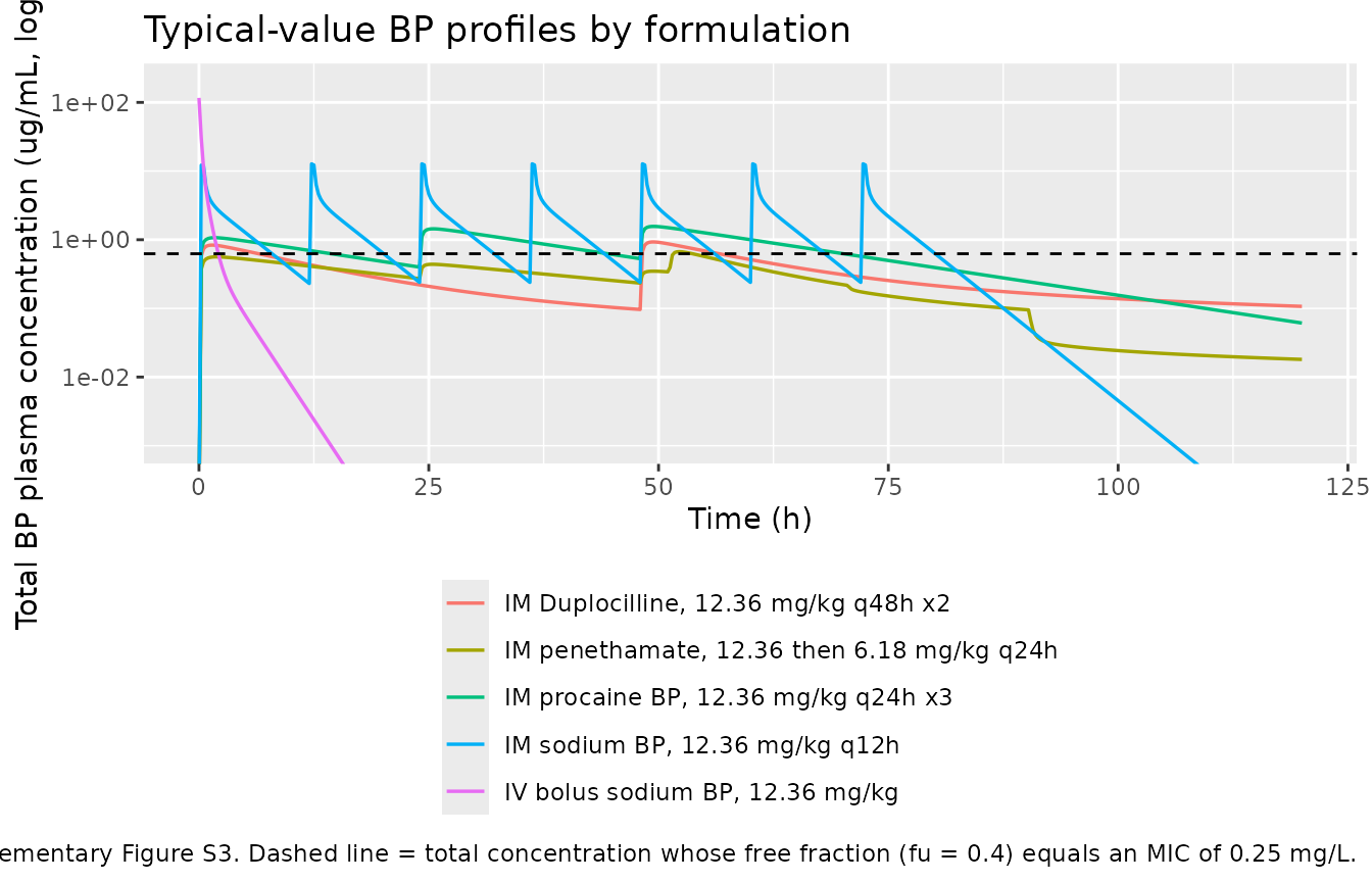

The flip-flop the authors emphasise is visible: every IM formulation has a terminal slope shallower than the 1.5 h IV terminal half-life, because absorption rather than elimination is rate-limiting.

The formulation-switched additive residual SD

Lallemand 2023 estimated a separate additive residual standard deviation for each of its five observation blocks (Supplementary Table S7, rows stdev0-stdev4) while sharing one multiplicative CV across all of them. The packaged model keeps a single Cc endpoint - the assay measures one analyte - and derives addSd from the FORM_BP_* indicator columns, so all five published values are retained. Every simulation above and below runs with sigma = NA (no residual noise added), so this check reads the derived addSd back out of the solution to confirm the switch selects the right block.

# No rounding here: addSd is computed from the same expression at every row, so
# it is bit-identical within an arm, and rounding would throw away digits the
# 1e-12 comparison below needs.
addsd_seen <- sim_arms |>
  group_by(arm) |>
  summarise(addSd = unique(addSd), .groups = "drop")
stopifnot(nrow(addsd_seen) == 5)  # one distinct value per arm, i.e. no mixing

published_addsd <- tibble::tribble(
  ~arm,                                          ~`Supp. Table S7`, ~row,
  "IV bolus sodium BP, 12.36 mg/kg",             0.00792812036590013, "stdev0",
  "IM sodium BP, 12.36 mg/kg q12h",              0.162677174710096,   "stdev1",
  "IM Duplocilline, 12.36 mg/kg q48h x2",        0.00653731719464946, "stdev2",
  "IM procaine BP, 12.36 mg/kg q24h x3",         0.00457902506048033, "stdev3",
  "IM penethamate, 12.36 then 6.18 mg/kg q24h",  0.00806824116414487, "stdev4"
)

chk_addsd <- left_join(published_addsd, addsd_seen, by = "arm")
stopifnot(!any(is.na(chk_addsd$addSd)))
stopifnot(isTRUE(all.equal(chk_addsd$addSd, chk_addsd$`Supp. Table S7`,
                           tolerance = 1e-12)))

chk_addsd |>
  transmute(Arm = arm, `Supplementary Table S7 row` = row,
            `Published SD (ug/mL)` = `Supp. Table S7`,
            `Selected by the model` = addSd) |>
  knitr::kable(caption = paste("The additive residual SD selected by the FORM_BP_*",
                               "indicators, against the five published values."))

The additive residual SD selected by the FORM_BP_* indicators, against the five published values.
Arm	Supplementary Table S7 row	Published SD (ug/mL)	Selected by the model
IV bolus sodium BP, 12.36 mg/kg	stdev0	0.0079281	0.0079281
IM sodium BP, 12.36 mg/kg q12h	stdev1	0.1626772	0.1626772
IM Duplocilline, 12.36 mg/kg q48h x2	stdev2	0.0065373	0.0065373
IM procaine BP, 12.36 mg/kg q24h x3	stdev3	0.0045790	0.0045790
IM penethamate, 12.36 then 6.18 mg/kg q24h	stdev4	0.0080682	0.0080682

Replicating the PK/PD cutoff analysis

The paper’s headline results are Monte Carlo quantiles of two PK/PD indices, computed with a free fraction of fu = 0.4:

fAUC/MIC in hours, with a pharmacodynamic target (PDT) equal to the treatment duration (72 h for a 3-day regimen, 96 h for the 48-h-interval Duplocilline regimen);
%fT>MIC, with a PDT of 30% or 40% of the dosing interval (21.6 h or 28.8 h over 72 h), or 90% of the infusion time (21.6 h over 24 h) for a continuous infusion.

The paper reports the Q90% quantile: the value that 90% of horses exceed, i.e. the 10th percentile of the simulated distribution. The PK/PD cutoff is the highest MIC whose Q90% still reaches the PDT.

The model integrates both indices as ODE states (auc_free and t_above_mic), exactly as the Phoenix deriv(AUC_...) / deriv(T_above_...) constructs did, so they can be read straight off the solution.

set.seed(20231025)
N_ARM <- 200L  # 200 per arm is the vignette cap; the paper used 5,000

proc_doses <- tibble(time = c(0, 24, 48), amt = DOSE, cmt = "depot2")
proc_arm_covs <- list(France = character(), Sweden = "STUDY_SWEDEN_IM",
                      USA1 = "STUDY_USA1", Japan = "STUDY_JAPAN")
sc_proc <- build_scenario(
  lapply(proc_arm_covs, function(s) {
    list(doses = proc_doses, obs = seq(0, 72, by = 0.5), set = c("FORM_BP_PROC", s))
  }),
  n = N_ARM
)

sim_proc <- solve_scenario(sc_proc)

Figure 7: fAUC/MIC for procaine BP

mic_grid <- c(0.0625, 0.1, 0.125, 0.25, 0.375, 0.5, 1, 2)

# fAUC/MIC scales exactly as 1/MIC, so one simulation serves every MIC.
end_proc <- sim_proc |> filter(time == 72) |> select(id, arm, auc_free)

fauc <- tidyr::expand_grid(end_proc, mic = mic_grid) |>
  mutate(index = auc_free / mic)

fauc_q <- fauc |>
  group_by(arm, mic) |>
  summarise(Mean = mean(index), `CV%` = 100 * sd(index) / mean(index),
            `Q90%` = quantile(index, 0.10), `Q50%` = median(index), .groups = "drop")

ggplot(fauc_q, aes(mic, `Q90%`, colour = arm)) +
  geom_line() + geom_point() +
  geom_hline(yintercept = 72, linetype = "dashed") +
  scale_x_continuous(trans = "log2", breaks = mic_grid) +
  scale_y_log10() +
  labs(x = "MIC (mg/L, log2 scale)", y = "Q90% of fAUC/MIC (h, log10 scale)",
       colour = "Dataset",
       title = "Figure 7 (left) - 90th quantile of fAUC/MIC vs MIC",
       caption = paste("Replicates Figure 7 of Lallemand 2023: procaine BP 12.36 mg/kg",
                       "q24h for 3 days. Dashed line = PDT of 72 h."))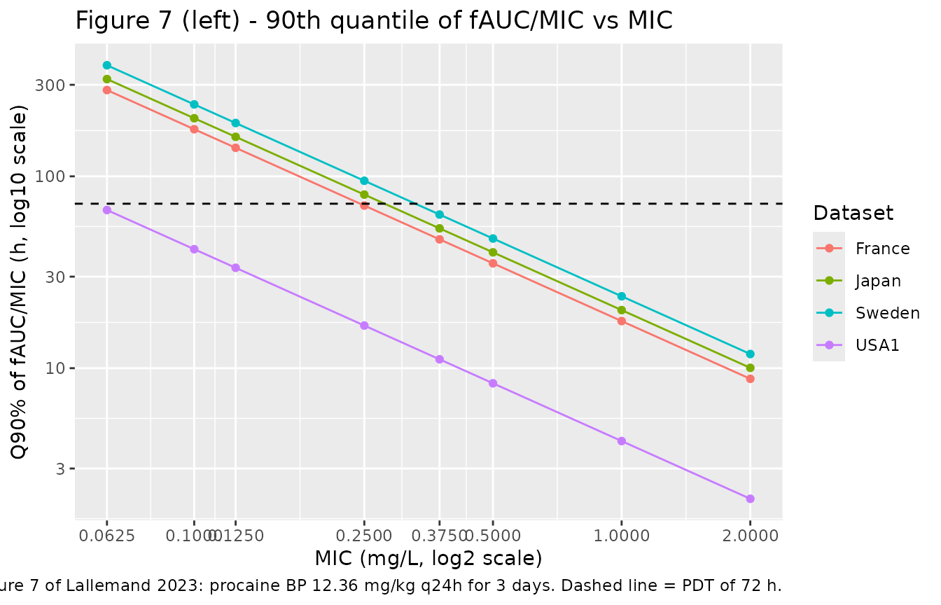

pta <- fauc |>
  group_by(arm, mic) |>
  summarise(PTA = 100 * mean(index >= 72), .groups = "drop")

ggplot(pta, aes(mic, PTA, colour = arm)) +
  geom_line() + geom_point() +
  geom_hline(yintercept = 90, linetype = "dashed") +
  scale_x_continuous(trans = "log2", breaks = mic_grid) +
  labs(x = "MIC (mg/L, log2 scale)", y = "Probability of target attainment (%)",
       colour = "Dataset",
       title = "Figure 7 (right) - PTA for a fAUC/MIC target of 72 h",
       caption = "Replicates Figure 7 of Lallemand 2023, right panel.")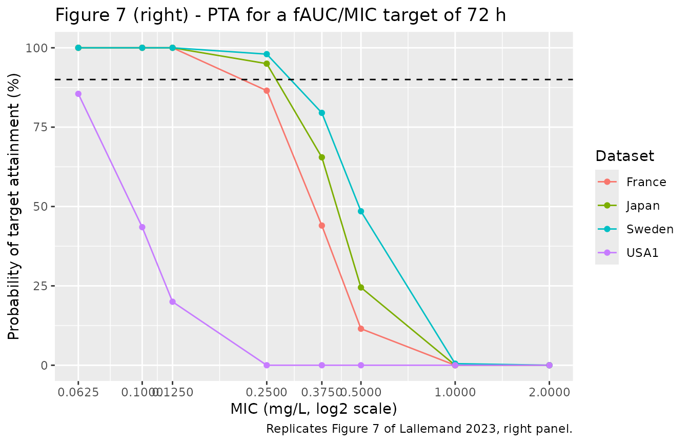

Comparison against the published Monte Carlo quantiles

Lallemand 2023 Supplementary Table S13 reports the mean, CV% and quantiles of fAUC/MIC (0-72 h) for the reference regimen. The mean and CV% are distributional summaries that converge quickly, so they carry strict tolerances; the Q90% quantile is a tail statistic and this vignette draws 200 horses per arm against the paper’s 5,000, so it carries a looser one.

published_s13 <- tibble::tribble(
  ~arm,     ~mic,   ~Mean, ~`CV%`, ~`Q90%`, ~`Q50%`,
  "France", 0.0625,  423,  28.70,  282,     406,
  "France", 0.1250,  211,  28.70,  141,     203,
  "France", 0.2500,  106,  28.70,   70.4,   102,
  "France", 0.5000,   52.8, 28.70,  35.2,    50.8,
  "Japan",  0.0625,  491,  28.31,  331,     474,
  "Japan",  0.2500,  123,  28.31,   82.7,   119,
  "Sweden", 0.0625,  585,  28.56,  391,     564,
  "Sweden", 0.2500,  146,  28.56,   97.9,   141,
  "USA1",   0.0625,  109,  40.62,   61,     102,
  "USA1",   0.2500,   27.4, 40.62,  15.2,    25.5
)

cmp_s13 <- published_s13 |>
  rename(Mean_pub = Mean, `CV%_pub` = `CV%`, `Q90%_pub` = `Q90%`, `Q50%_pub` = `Q50%`) |>
  left_join(fauc_q, by = c("arm", "mic")) |>
  mutate(`Mean diff %` = 100 * (Mean - Mean_pub) / Mean_pub,
         `CV diff %`   = 100 * (`CV%` - `CV%_pub`) / `CV%_pub`,
         `Q90 diff %`  = 100 * (`Q90%` - `Q90%_pub`) / `Q90%_pub`,
         `Q50 diff %`  = 100 * (`Q50%` - `Q50%_pub`) / `Q50%_pub`)

# STRICT on the fast-converging summaries; looser on the tail quantile (n = 200 vs 5,000).
stopifnot(all(abs(cmp_s13$`Mean diff %`) < 5))
stopifnot(all(abs(cmp_s13$`Q50 diff %`) < 5))
stopifnot(all(abs(cmp_s13$`CV diff %`)  < 15))
stopifnot(all(abs(cmp_s13$`Q90 diff %`) < 15))
# The USA1 dataset must stand out with a markedly higher CV% than the other three,
# because its very slow absorption (MAT 230 h) makes AUC(0-72 h) depend on Ka as
# well as on CL (Lallemand 2023 Discussion).
stopifnot(min(cmp_s13$`CV%`[cmp_s13$arm == "USA1"]) >
            max(cmp_s13$`CV%`[cmp_s13$arm != "USA1"]))

cmp_s13 |>
  transmute(Dataset = arm, `MIC (mg/L)` = mic,
            `Mean sim` = signif(Mean, 4), `Mean pub` = Mean_pub,
            `CV% sim` = signif(`CV%`, 3), `CV% pub` = `CV%_pub`,
            `Q90% sim` = signif(`Q90%`, 4), `Q90% pub` = `Q90%_pub`,
            `Q90 diff %` = round(`Q90 diff %`, 1)) |>
  knitr::kable(caption = paste("fAUC/MIC (0-72 h) for procaine BP 12.36 mg/kg q24h x3,",
                               "simulated (200 horses/arm) vs Lallemand 2023",
                               "Supplementary Table S13 (5,000 horses/arm)."))

fAUC/MIC (0-72 h) for procaine BP 12.36 mg/kg q24h x3, simulated (200 horses/arm) vs Lallemand 2023 Supplementary Table S13 (5,000 horses/arm).
Dataset	MIC (mg/L)	Mean sim	Mean pub	CV% sim	CV% pub	Q90% sim	Q90% pub	Q90 diff %
France	0.0625	426.30	423.0	28.1	28.70	281.60	282.0	-0.1
France	0.1250	213.10	211.0	28.1	28.70	140.80	141.0	-0.1
France	0.2500	106.60	106.0	28.1	28.70	70.41	70.4	0.0
France	0.5000	53.29	52.8	28.1	28.70	35.20	35.2	0.0
Japan	0.0625	495.50	491.0	29.1	28.31	321.30	331.0	-2.9
Japan	0.2500	123.90	123.0	29.1	28.31	80.32	82.7	-2.9
Sweden	0.0625	588.40	585.0	30.1	28.56	379.30	391.0	-3.0
Sweden	0.2500	147.10	146.0	30.1	28.56	94.83	97.9	-3.1
USA1	0.0625	113.00	109.0	39.7	40.62	66.74	61.0	9.4
USA1	0.2500	28.26	27.4	39.7	40.62	16.68	15.2	9.8

The reproduction places the PK/PD cutoff exactly where the paper does: 0.25 mg/L for the French, Swedish and Japanese formulations, and one to two dilutions lower for USA1.

cutoff <- fauc_q |>
  filter(`Q90%` >= 72) |>
  group_by(arm) |>
  summarise(`PK/PD cutoff (mg/L)` = max(mic), .groups = "drop")
knitr::kable(cutoff, caption = paste("Highest MIC whose Q90% fAUC/MIC still reaches the",
                                     "72 h PDT (Lallemand 2023 Section 3.4)."))

Highest MIC whose Q90% fAUC/MIC still reaches the 72 h PDT (Lallemand 2023 Section 3.4).
arm	PK/PD cutoff (mg/L)
France	0.125
Japan	0.250
Sweden	0.250

Note the marginal case the paper’s own table contains: for France the published Q90% at MIC 0.25 mg/L is 70.4 h, 2.2% below the 72 h PDT, yet the paper reports the cutoff as 0.25 mg/L (read off the Figure 7 curve and rounded to the nearest two-fold dilution). Japan (82.7 h) and Sweden (97.9 h) clear the PDT outright. The table above therefore reproduces the paper’s numbers; whether France’s 0.25 mg/L cutoff is called at 70.4 h or at 72 h is the paper’s editorial rounding, not a property of the model.

Figure 8: fT>MIC for procaine BP

fT>MIC cannot be rescaled from a single run, so this section re-solves the cohort once per MIC by overriding the mic parameter.

mic_tmic <- c(0.0625, 0.125, 0.25, 0.5, 1)
tmic <- bind_rows(lapply(mic_tmic, function(m) {
  solve_scenario(sc_proc, mic = m) |>
    filter(time == 72) |>
    transmute(id, arm, mic = m, t_above = t_above_mic)
}))

tmic_q <- tmic |>
  group_by(arm, mic) |>
  summarise(`Q90%` = quantile(t_above, 0.10), Median = median(t_above), .groups = "drop")

ggplot(tmic_q, aes(mic, `Q90%`, colour = arm)) +
  geom_line() + geom_point() +
  geom_hline(yintercept = c(21.6, 28.8), linetype = c("dashed", "dotted")) +
  scale_x_continuous(trans = "log2", breaks = mic_tmic) +
  labs(x = "MIC (mg/L, log2 scale)", y = "Q90% of cumulative fT>MIC over 72 h (h)",
       colour = "Dataset",
       title = "Figure 8 - 90th quantile of fT>MIC vs MIC",
       caption = paste("Replicates Figure 8 of Lallemand 2023. Dashed = 30% of the",
                       "dosing interval (21.6 h); dotted = 40% (28.8 h)."))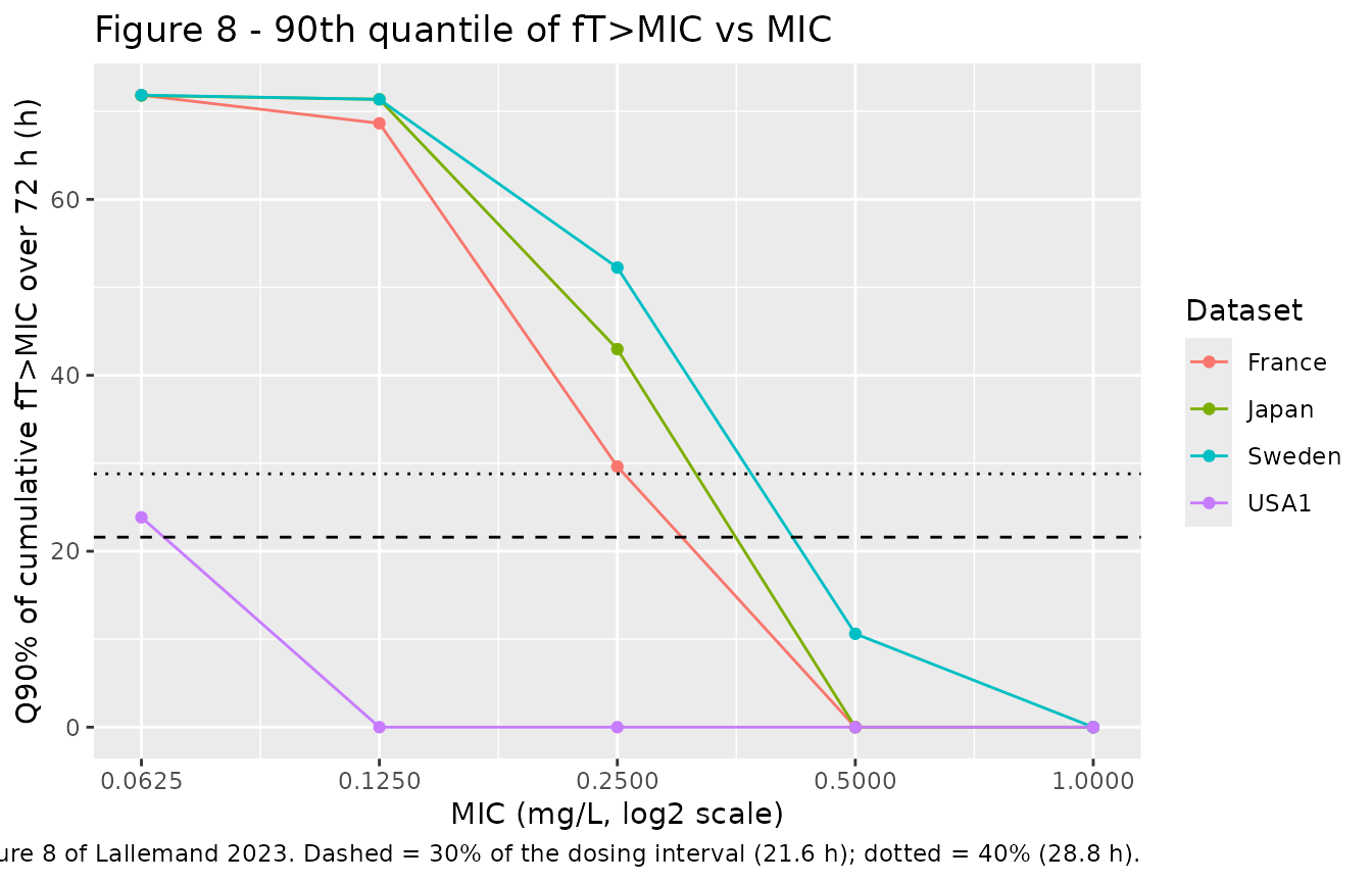

cutoff_tmic <- tmic_q |>
  filter(`Q90%` >= 21.6) |>
  group_by(arm) |>
  summarise(`fT>MIC cutoff at 30% (mg/L)` = max(mic), .groups = "drop")

# Lallemand 2023 Section 3.4: with fT>MIC and a 30% or 40% PDT the cutoff is
# again 0.25 mg/L for France, Sweden and Japan, and 0.0625 mg/L for USA1.
expected <- c(France = 0.25, Japan = 0.25, Sweden = 0.25, USA1 = 0.0625)
got <- setNames(cutoff_tmic$`fT>MIC cutoff at 30% (mg/L)`, cutoff_tmic$arm)
stopifnot(identical(sort(names(got)), sort(names(expected))))
stopifnot(all(got[names(expected)] == expected))
# No procaine formulation may reach the 30% target at an MIC of 0.5 mg/L
# ("no procaine BP formulation reached the PDT of 30% for an MIC of 0.50 mg/L").
stopifnot(all(tmic_q$`Q90%`[tmic_q$mic == 0.5] < 21.6))

knitr::kable(cutoff_tmic, caption = paste("fT>MIC PK/PD cutoffs, reproducing Lallemand",
                                          "2023 Section 3.4 and Figure 8."))

fT>MIC PK/PD cutoffs, reproducing Lallemand 2023 Section 3.4 and Figure 8.
arm	fT>MIC cutoff at 30% (mg/L)
France	0.2500
Japan	0.2500
Sweden	0.2500
USA1	0.0625

Duplocilline and penethamate (Supplementary Tables S14, S15)

Both long-acting formulations fail to reach the 0.25 mg/L cutoff; the paper concludes 0.0625 mg/L for each.

sc_la <- build_scenario(list(
  Duplocilline = list(
    doses = bind_rows(tibble(time = c(0, 48), amt = DOSE, cmt = "depot3"),
                      tibble(time = c(0, 48), amt = DOSE, cmt = "depot4")),
    obs = seq(0, 96, by = 0.5), set = "FORM_BP_DUPLO"),
  Penethamate = list(
    doses = tibble(time = c(0, 24, 48), amt = c(DOSE, DOSE / 2, DOSE / 2),
                   cmt = c("depot5", "depot6", "depot7")),
    obs = seq(0, 72, by = 0.5), set = "FORM_BP_PENETH")
), n = N_ARM)

sim_la <- solve_scenario(sc_la)

# Duplocilline is assessed over 96 h with a PDT of 96 h; penethamate over 72 h / 72 h.
la_end <- bind_rows(
  sim_la |> filter(arm == "Duplocilline", time == 96) |> mutate(pdt = 96),
  sim_la |> filter(arm == "Penethamate",  time == 72) |> mutate(pdt = 72)
) |>
  select(id, arm, pdt, auc_free)

la_q <- tidyr::expand_grid(la_end, mic = mic_grid) |>
  mutate(index = auc_free / mic) |>
  group_by(arm, pdt, mic) |>
  summarise(Mean = mean(index), `CV%` = 100 * sd(index) / mean(index),
            `Q90%` = quantile(index, 0.10), .groups = "drop")

published_la <- tibble::tribble(
  ~arm,            ~mic,   ~Mean_pub, ~`CV%_pub`, ~`Q90%_pub`,
  "Duplocilline",  0.0625, 208,       42.00,      101,
  "Duplocilline",  0.2500,  52.1,     42.00,       25.3,
  "Penethamate",   0.0625, 173,       33.24,      106,
  "Penethamate",   0.2500,  43.4,     33.24,       26.5
)

cmp_la <- published_la |>
  left_join(la_q, by = c("arm", "mic")) |>
  mutate(`Mean diff %` = 100 * (Mean - Mean_pub) / Mean_pub,
         `CV diff %`   = 100 * (`CV%` - `CV%_pub`) / `CV%_pub`,
         `Q90 diff %`  = 100 * (`Q90%` - `Q90%_pub`) / `Q90%_pub`)

stopifnot(all(abs(cmp_la$`Mean diff %`) < 5))
stopifnot(all(abs(cmp_la$`CV diff %`)  < 15))
stopifnot(all(abs(cmp_la$`Q90 diff %`) < 20))

# The paper's conclusions, as assertions.
la_cut <- la_q |> filter(`Q90%` >= pdt) |> group_by(arm) |>
  summarise(cutoff = max(mic), .groups = "drop")
stopifnot(nrow(la_cut) == 2)
stopifnot(all(la_cut$cutoff == 0.0625))

cmp_la |>
  transmute(Formulation = arm, `MIC (mg/L)` = mic, `PDT (h)` = pdt,
            `Mean sim` = signif(Mean, 4), `Mean pub` = Mean_pub,
            `CV% sim` = signif(`CV%`, 3), `CV% pub` = `CV%_pub`,
            `Q90% sim` = signif(`Q90%`, 4), `Q90% pub` = `Q90%_pub`,
            `Q90 diff %` = round(`Q90 diff %`, 1)) |>
  knitr::kable(caption = paste("fAUC/MIC for the two long-acting formulations, simulated",
                              "vs Lallemand 2023 Supplementary Tables S14 (Duplocilline,",
                              "12.36 mg/kg q48h x2) and S15 (penethamate, 12.36 then",
                              "6.18 mg/kg q24h)."))

fAUC/MIC for the two long-acting formulations, simulated vs Lallemand 2023 Supplementary Tables S14 (Duplocilline, 12.36 mg/kg q48h x2) and S15 (penethamate, 12.36 then 6.18 mg/kg q24h).
Formulation	MIC (mg/L)	PDT (h)	Mean sim	Mean pub	CV% sim	CV% pub	Q90% sim	Q90% pub	Q90 diff %
Duplocilline	0.0625	96	203.80	208.0	39.4	42.00	107.00	101.0	5.9
Duplocilline	0.2500	96	50.96	52.1	39.4	42.00	26.74	25.3	5.7
Penethamate	0.0625	72	174.00	173.0	34.3	33.24	107.00	106.0	1.0
Penethamate	0.2500	72	43.50	43.4	34.3	33.24	26.76	26.5	1.0

IV 24-hour continuous infusion (Supplementary Table S20)

inf_doses <- tibble(time = 0, amt = DOSE, cmt = "central", rate = DOSE / 24)
sc_inf <- build_scenario(
  lapply(list(France = character(), Sweden = "STUDY_SWEDEN_IV", USA2 = "STUDY_USA2"),
         function(s) list(doses = inf_doses, obs = seq(0, 24, by = 0.5), set = s)),
  n = N_ARM
)

inf_q <- bind_rows(lapply(c(0.0625, 0.25, 0.5), function(m) {
  solve_scenario(sc_inf, mic = m) |>
    filter(time == 24) |>
    group_by(arm) |>
    summarise(mic = m, Mean = mean(t_above_mic),
              `Q90%` = quantile(t_above_mic, 0.10), .groups = "drop")
}))

published_s20 <- tibble::tribble(
  ~arm,     ~mic,   ~Mean_pub, ~`Q90%_pub`,
  "France", 0.0625, 23.9,      23.8,
  "Sweden", 0.0625, 23.9,      23.8,
  "USA2",   0.0625, 23.9,      23.8,
  "France", 0.2500, 23.0,      22.5,
  "Sweden", 0.2500, 23.7,      23.2,
  "USA2",   0.2500, 23.5,      22.9,
  "France", 0.5000,  6.1,       0.0,
  "Sweden", 0.5000, 22.5,      21.1,
  "USA2",   0.5000, 15.2,       0.0
)

cmp_inf <- published_s20 |> left_join(inf_q, by = c("arm", "mic"))
lo <- cmp_inf$mic <= 0.25   # rows where the distribution is not bimodal

# Section 3.4: "for an MIC of 0.25 mg/L, 24-h infusions of a total dose of
# 12.36 mg/kg were found to maintain BP plasma concentrations above this MIC for
# more than 22 h out of the 24-h infusion for 90% of the horses across the three
# datasets examined (France, Sweden and USA2)."
stopifnot(all(cmp_inf$`Q90%`[cmp_inf$mic == 0.25] > 22))

# At MIC 0.5, "only the Swedish horses were able to maintain values above this
# MIC for 21 h". Note that 21 h is itself BELOW the 21.6 h PDT, so this is not a
# claim that Sweden attains the target - it is a claim that Sweden alone comes
# close while France and USA2 collapse to a Q90% of zero.
sw <- cmp_inf$`Q90%`[cmp_inf$mic == 0.5 & cmp_inf$arm == "Sweden"]
other <- cmp_inf$`Q90%`[cmp_inf$mic == 0.5 & cmp_inf$arm != "Sweden"]
stopifnot(abs(sw - 21.1) / 21.1 < 0.10, all(other == 0))

# Means and Q90% agree closely wherever the distribution is unimodal. The
# MIC 0.5 rows for France and USA2 are excluded from the mean check because
# their fT>MIC distributions are strongly bimodal there (published CV% 166 and
# 71), so a 200-horse mean is dominated by how many draws land above zero.
stopifnot(all(abs(100 * (cmp_inf$Mean[lo] - cmp_inf$Mean_pub[lo]) /
                    cmp_inf$Mean_pub[lo]) < 5))
stopifnot(all(abs(cmp_inf$`Q90%`[lo] - cmp_inf$`Q90%_pub`[lo]) < 1))

cmp_inf |>
  transmute(Dataset = arm, `MIC (mg/L)` = mic,
            `Mean sim (h)` = signif(Mean, 4), `Mean pub (h)` = Mean_pub,
            `Q90% sim (h)` = signif(`Q90%`, 4), `Q90% pub (h)` = `Q90%_pub`) |>
  knitr::kable(caption = paste("Cumulative fT>MIC over a 24 h IV infusion of 12.36 mg/kg,",
                               "simulated vs Lallemand 2023 Supplementary Table S20.",
                               "PDT = 21.6 h (90% of the infusion)."))

Cumulative fT>MIC over a 24 h IV infusion of 12.36 mg/kg, simulated vs Lallemand 2023 Supplementary Table S20. PDT = 21.6 h (90% of the infusion).
Dataset	MIC (mg/L)	Mean sim (h)	Mean pub (h)	Q90% sim (h)	Q90% pub (h)
France	0.0625	23.940	23.9	23.88	23.8
Sweden	0.0625	23.940	23.9	23.85	23.8
USA2	0.0625	23.930	23.9	23.86	23.8
France	0.2500	23.030	23.0	22.15	22.5
Sweden	0.2500	23.640	23.7	23.04	23.2
USA2	0.2500	22.940	23.5	22.43	22.9
France	0.5000	6.799	6.1	0.00	0.0
Sweden	0.5000	22.080	22.5	20.57	21.1
USA2	0.5000	10.480	15.2	0.00	0.0

PKNCA validation

NCA is run with PKNCA on typical-value profiles for the four single-dose IV datasets, so the results can be compared with the paper’s own non-compartmental analysis.

nca_grid <- c(seq(0, 2, by = 0.02), seq(2.25, 24, by = 0.25))
sc_nca <- build_scenario(
  lapply(list(France = character(), Sweden = "STUDY_SWEDEN_IV",
              USA1 = "STUDY_USA1", USA2 = "STUDY_USA2"),
         function(s) list(doses = tibble(time = 0, amt = DOSE, cmt = "central"),
                          obs = nca_grid, set = s))
)
sim_nca_raw <- solve_scenario(sc_nca, typical = TRUE)

sim_nca <- sim_nca_raw |>
  filter(!is.na(Cc)) |>
  select(id, time, Cc, arm)

# Guarantee a time = 0 record per (id, arm) so PKNCA can anchor AUC from 0.
sim_nca <- bind_rows(
  sim_nca,
  sim_nca |> distinct(id, arm) |> mutate(time = 0, Cc = 0)
) |>
  distinct(id, arm, time, .keep_all = TRUE) |>
  arrange(id, arm, time)

conc_obj <- PKNCA::PKNCAconc(as.data.frame(sim_nca), Cc ~ time | arm + id)

dose_df <- sc_nca$events |>
  filter(evid == 1) |>
  left_join(sc_nca$map, by = "id") |>   # one row per id in `map`, so no fan-out
  select(id, time, amt, arm) |>
  as.data.frame()
dose_obj <- PKNCA::PKNCAdose(dose_df, amt ~ time | arm + id)

intervals <- data.frame(start = 0, end = Inf,
                        cmax = TRUE, tmax = TRUE, auclast = TRUE,
                        aucinf.obs = TRUE, half.life = TRUE, cl.obs = TRUE)

nca_res <- PKNCA::pk.nca(PKNCA::PKNCAdata(conc_obj, dose_obj, intervals = intervals))

nca_wide <- as.data.frame(nca_res) |>
  filter(start == 0, is.infinite(end)) |>   # drop PKNCA dependency rows
  select(arm, PPTESTCD, PPORRES) |>
  tidyr::pivot_wider(names_from = PPTESTCD, values_from = PPORRES)

# Mass-balance gate: for an IV bolus, AUCinf must equal Dose / CL exactly, and the
# PKNCA-derived clearance must recover the model's own dataset-specific CL.
model_cl <- c(France = cl,
              Sweden = cl * exp(g("e_study_sweden_iv_cl")),
              USA1   = cl * exp(g("e_study_usa1_cl")),
              USA2   = cl * exp(g("e_study_usa2_cl")))
nca_wide$cl_model <- model_cl[as.character(nca_wide$arm)]
stopifnot(all(abs(100 * (nca_wide$cl.obs - nca_wide$cl_model) / nca_wide$cl_model) < 1))
stopifnot(all(abs(100 * (nca_wide$aucinf.obs - DOSE / nca_wide$cl_model) /
                    (DOSE / nca_wide$cl_model)) < 1))

nca_wide |>
  transmute(Dataset = arm, `Cmax (ug/mL)` = signif(cmax, 4),
            `Tmax (h)` = signif(tmax, 3),
            `AUClast (ug*h/mL)` = signif(auclast, 4),
            `AUCinf (ug*h/mL)` = signif(aucinf.obs, 4),
            `t1/2 (h)` = signif(half.life, 3),
            `CL from NCA (mL/kg/h)` = signif(cl.obs, 4),
            `CL in model (mL/kg/h)` = signif(cl_model, 4)) |>
  knitr::kable(caption = paste("PKNCA on typical-value IV bolus profiles (12.36 mg/kg).",
                               "The NCA clearance recovers each dataset's model CL to",
                               "<1%, confirming dose / volume / clearance unit",
                               "consistency (ug/kg dosed, mL/kg volumes, ug/mL",
                               "concentrations)."))

PKNCA on typical-value IV bolus profiles (12.36 mg/kg). The NCA clearance recovers each dataset’s model CL to <1%, confirming dose / volume / clearance unit consistency (ug/kg dosed, mL/kg volumes, ug/mL concentrations).
Dataset	Cmax (ug/mL)	AUClast (ug*h/mL)	AUCinf (ug*h/mL)	t1/2 (h)	CL from NCA (mL/kg/h)	CL in model (mL/kg/h)
France	116.4	25.71	25.71	1.48	480.8	480.9
Sweden	116.4	50.91	50.91	1.59	242.8	242.8
USA1	116.4	29.15	29.15	1.49	424.0	424.1
USA2	116.4	29.45	29.45	1.49	419.6	419.7

Comparison against the published NCA

Lallemand 2023 Table 2 reports a non-compartmental analysis of the observed IV data. This is not a like-for-like comparison with the population model and the paper says so explicitly: the NCA was performed only “to obtain an initial estimate of basic pharmacokinetic parameters” that seeded the population fit (Section 2.2).

# Table 2 reports the observed-data NCA (means) for the three analysable IV
# datasets. Table 3 reports observed AUC(0-tlast) already scaled to the
# reference 12.36 mg/kg dose, which is the like-for-like AUC comparator (Table
# 2's AUCINF is at each dataset's actual dose, and the Swedish doses ranged
# 16.44-25.11 mg/kg).
published_nca <- tibble::tribble(
  ~arm,     ~cl_nca, ~cmax_nca, ~auc_nca_scaled, ~hl_nca,
  "France",  564,     79.0,     22.12,           1.49,
  "Sweden",  423,    117.0,     44.33,           1.28,
  "USA2",    300,    145.0,     44.49,           0.955
)

cmp_nca <- published_nca |>
  left_join(nca_wide |> mutate(arm = as.character(arm)) |>
              select(arm, cmax, aucinf.obs, half.life, cl_model), by = "arm") |>
  transmute(Dataset = arm,
            `CL model` = signif(cl_model, 4), `CL NCA` = cl_nca,
            `CL diff %` = round(100 * (cl_model - cl_nca) / cl_nca, 1),
            `AUCinf model` = signif(aucinf.obs, 4), `AUC NCA (scaled)` = auc_nca_scaled,
            `AUC diff %` = round(100 * (aucinf.obs - auc_nca_scaled) / auc_nca_scaled, 1),
            `t1/2 model` = signif(half.life, 3), `t1/2 NCA` = hl_nca,
            `t1/2 diff %` = round(100 * (half.life - hl_nca) / hl_nca, 1),
            `Cmax model` = signif(cmax, 4), `Cmax NCA` = cmax_nca)

# For an IV dose AUCinf = Dose / CL exactly, so the model's AUC column is a pure
# restatement of its CL column -- that identity is asserted in the PKNCA chunk
# above (< 1%). It CANNOT be asserted between the model and the published NCA,
# because Table 2's per-dataset mean CL and mean AUCINF are themselves not
# mutually consistent: they are arithmetic means of reciprocally related
# quantities, and mean(D / AUC_i) != mean(D) / mean(AUC_i) once the individual
# spread is large. The Swedish row makes this unmissable, so it is reported
# rather than asserted.
sweden_implied_cl <- 20.87e3 / 70.4  # mean Swedish IV dose (Table S2) / mean AUCINF (Table 2)
cat(sprintf(paste("Table 2 Sweden: mean CL = 423 mL/kg/h, but mean dose / mean AUCINF",
                  "= %.0f mL/kg/h (CV%% of the 4 individual clearances = 86%%).\n"),
            sweden_implied_cl))
#> Table 2 Sweden: mean CL = 423 mL/kg/h, but mean dose / mean AUCINF = 296 mL/kg/h (CV% of the 4 individual clearances = 86%).

knitr::kable(cmp_nca, caption = paste("Typical-value model NCA vs the observed-data NCA of",
                                      "Lallemand 2023 Table 2 (clearance, Cmax, half-life)",
                                      "and Table 3 (AUC scaled to 12.36 mg/kg). All means.",
                                      "Differences are expected and explained below - the",
                                      "two analyses estimate different things."))

Typical-value model NCA vs the observed-data NCA of Lallemand 2023 Table 2 (clearance, Cmax, half-life) and Table 3 (AUC scaled to 12.36 mg/kg). All means. Differences are expected and explained below - the two analyses estimate different things.
Dataset	CL model	CL NCA	CL diff %	AUCinf model	AUC NCA (scaled)	AUC diff %	t1/2 model	t1/2 NCA	t1/2 diff %	Cmax model	Cmax NCA
France	480.9	564	-14.7	25.71	22.12	16.2	1.48	1.490	-0.7	116.4	79
Sweden	242.8	423	-42.6	50.91	44.33	14.8	1.59	1.280	24.3	116.4	117
USA2	419.7	300	39.9	29.45	44.49	-33.8	1.49	0.955	56.5	116.4	145

The differences here are structural, not defects, and they reduce to two causes that the paper itself identifies.

1. Every AUC difference is a clearance difference. For an IV dose, AUCinf = Dose / CL exactly, so the model’s AUC column is a pure restatement of its clearance column (the PKNCA chunk above asserts that identity to <1%). The question is therefore only why the population clearances (481 / 243 / 420 mL/kg/h for France / Sweden / USA2) differ from the NCA clearances (564 / 423 / 300). The paper’s answer is the third disposition phase: the low French limit of quantification (10 ng/mL) let the population model resolve a terminal gamma phase (half-life 1.48 h) that a linear-trapezoidal NCA truncates. Truncation biases NCA clearance upward for France (564 vs 481), whose concentrations were followed longest, and downward for USA2 (300 vs 420), whose last quantifiable sample was at 6 h and whose animals the authors treated as censored between 6 and 8 h. This is precisely the paper’s central methodological argument for a 3-compartment population model over the 2-compartment models fitted in the original single-site publications (Discussion).

Sweden is a special case, and the two published columns cannot both be matched because they are not mutually consistent with each other. Table 2 gives a mean Swedish clearance of 423 mL/kg/h, but the mean Swedish dose divided by the mean Swedish AUCINF is only about 296 mL/kg/h - arithmetic means of reciprocally related quantities do not commute, and the four individual Swedish clearances span 162-953 mL/kg/h (CV 86%). The population estimate of 243 mL/kg/h is closer to the exposure-weighted value than to the arithmetic mean of the individual clearances. This is a property of how Table 2 summarises four very heterogeneous horses, not a defect in either analysis.

2. The Cmax and half-life columns mostly measure heterogeneity the model deliberately does not carry. The 'source of dataset' covariate acts on clearance only, so the model’s Cmax is Dose / Vc = 116.4 ug/mL for every dataset, whereas the observed Cmax ranges from 79 (France) to 145 ug/mL (USA2). Between-dataset differences in distribution volume are absorbed into the very large Vc between-subject variability (174%) rather than into a covariate - a deliberate choice, since the paper’s objective was a cutoff generic across the whole equine population, and Table 2 shows the volume differences are what compensate the clearance differences (“the half-life was relatively similar for horses in each of the three datasets, the differences in clearance being largely compensated for by differences in the volumes of distribution”). The model’s terminal half-life is likewise dataset-invariant at 1.48-1.59 h and cannot track the NCA’s 0.955-1.49 h spread.

Two further points worth keeping in view when reading the Swedish row: Table 2’s Swedish NCA pooled doses of 16.44-25.11 mg/kg (Supplementary Table S2), which is why the dose-scaled Table 3 value is used here rather than Table 2’s raw AUCINF; and the Swedish NCA CV% is 47-86% because 3 of the 4 Swedish IV horses had markedly higher profiles than the fourth, for reasons the authors state remain unexplained.

No parameter was adjusted to narrow any of these gaps.

Assumptions and deviations

All parameter values come from the paper or its open-access supplement. Nothing was digitised from a figure, obtained by correspondence, or carried from another model. Main-text Table 6 is explicitly “a selection” of typical values; the complete set was taken from Supplementary Table S7 and the Phoenix control stream in Supplementary Data 2, and every value was cross-checked against the derived quantities in Supplementary Table S8 (see the verification table above).
Which covariate coefficients are fixed(). The paper prose (Sections 2.2 and 3.3) states that the clearance covariates for the Swedish IV, USA1 and USA2 cohorts were frozen at their IV-only values, while those for Japan and the Swedish IM cohort were estimated indirectly by a Bayesian method because neither cohort received an IV dose. The (freeze) flags in Supplementary Data 2 disagree: they mark Japan frozen and USA2 free. The prose is followed here, because the numeric precision of the published values independently confirms it - the three frozen coefficients appear to 6 decimal places and match Table 4’s IV-model estimates exactly, whereas the two Bayesian coefficients appear to 15 decimal places (full estimator output). The (freeze) flags on those two lines of the control stream appear to have been transposed.
Duplicated USA2 covariate term in the published Phoenix code. Supplementary Data 2 writes exp(dCldNationcode4*(Nationcode==4)) twice in the stparm(Cl = ...) expression. The packaged model applies it once. A single application gives 481 * exp(-0.136097) = 420 mL/kg/h, matching Table 4, Table 6 and Supplementary Tables S7 and S8, and the Discussion’s “87% of the reference value”; a doubled term would give 366 mL/kg/h (76%), contradicting all four. This is treated as a copy-paste error in the published code.
Bioavailability transform differs by formulation, as published. Equation 3 states that “for all IM formulations, bioavailability was estimated using an ilogit transformation”. Supplementary Data 2 applies ilogit to procaine BP, both Duplocilline components and penethamate, but uses a plain multiplicative model for IM sodium BP (stparm(FPeniNa = tvFPeniNa * exp(nFPeniNa))). The control stream is followed. One consequence is that a large positive etalfdepot_im_na draw can push the sodium BP bioavailability above 1; this is a property of the published parameterisation, not of the translation.
Unusual covariate form on procaine bioavailability. The dataset effect multiplies the logit-scale typical value before the inverse logit is taken, rather than being added on the logit scale: F = ilogit(tvFPROC * exp(dF * I(dataset)) + eta). This is reproduced exactly; it is confirmed by all four published bioavailabilities (99.960%, 99.960%, 99.974%, 99.999%) agreeing to five significant figures.
Sequential absorption is implemented with tad() rather than hard-coded dose times. Supplementary Data 2 encodes the rapid-to-slow switch with sequence{} blocks that enumerate the actual study dose times (seven 12-hourly sodium BP doses; penethamate at 0, 24 and 48 h). Using tad(<depot>) reproduces the same behaviour for those regimens while remaining valid for any other regimen a user simulates. Verified: the sodium BP rate constant is 1.0242 /h at 0.1 h and 0.4 h after a dose and 0.2481 /h at 0.6 h and 5 h, switching exactly at the fitted lag time of 0.471 h.
Penethamate injection sites are separate depots. The paper models three injection sites with different absorption kinetics, which means the packaged model expects the three penethamate doses to be given to depot5, depot6 and depot7 respectively. A fourth or later penethamate dose has no site of its own; the published model does not cover regimens longer than three administrations.
One residual-error endpoint with a formulation-switched additive SD. The paper estimated a separate additive residual standard deviation for each of its five observation blocks (Supplementary Table S7, stdev0-stdev4) while sharing one multiplicative CV of 0.283 across all of them. Because the assay measures a single analyte, the packaged model keeps one endpoint (Cc) and selects the additive SD from the FORM_BP_* indicator columns, so all five published values are retained and used. The FORM_BP_* covariates are therefore observation-level, not subject-level.
Weight-normalised units. Volumes are mL/kg and clearances mL/kg/h exactly as published, so doses must be supplied in ug/kg (12,360 ug/kg = 12.36 mg/kg = 22,000 IU/kg) for concentrations to come out in ug/mL. The PKNCA gate above confirms the unit chain by recovering each dataset’s model clearance from the simulated profile to within 1%.
No biological covariates. The paper deliberately excluded body weight, age, sex and breed so that the resulting PK/PD cutoff would apply to the whole equine population. The packaged model therefore has no allometric scaling; do not add any when simulating.
Monte Carlo cohort size. The paper used 5,000 simulated horses per scenario. This vignette uses 200 per arm to stay inside the package’s rendering budget, which is why the Q90% tail quantiles carry 15-20% tolerances while the means, medians and CV% carry 5-15% tolerances. Increasing N_ARM tightens the tail agreement.
fu is applied as a constant. Free concentrations are total concentrations scaled by 0.4, with no variability on fu. The paper does the same and notes in the Discussion that this makes the resulting cutoff conservative, because it attributes to fu a source of variability that does not exist.
Typographical issues in the published tables, noted but not acted on. Supplementary Table S15 lists the penethamate loading dose as 12360, 12361, 12362 … 12367 ug/kg across successive MIC rows; these are plainly all 12,360 ug/kg, since fAUC/MIC for a fixed regimen must scale exactly as 1/MIC (and the tabulated values do). Supplementary Table S2 gives the penethamate SPC dose as 11.91 then 5.96 mg/kg for a 500 kg horse, whereas the Monte Carlo simulations of Supplementary Table S15 use the reference 12.36 then 6.18 mg/kg; this vignette uses the simulation doses when comparing against Supplementary Table S15.