Brigatinib exposure-response in first-line ALK-positive NSCLC (Gupta 2022)
Source:vignettes/articles/Gupta_2022_brigatinib_exposure_response.Rmd
Gupta_2022_brigatinib_exposure_response.RmdGupta N, Reckamp KL, Camidge DR, Kleijn HJ, Ouerdani A, Bellanti F, Maringwa J, Hanley MJ, Wang S, Zhang P, Venkatakrishnan K. Population pharmacokinetic and exposure-response analyses from ALTA-1L: Model-based analyses supporting the brigatinib dose in ALK-positive NSCLC. Clin Transl Sci. 2022;15:1143-1154. doi:10.1111/cts.13231
ALTA-1L compared the ALK tyrosine kinase inhibitor brigatinib (180 mg
once daily after a 7-day lead-in at 90 mg) with crizotinib in
ALK-inhibitor-naive ALK-positive non-small cell lung cancer. Gupta 2022
did not fit a new pharmacokinetic model: it applied the
previously published brigatinib population PK model “without
modification” by Bayesian re-estimation to derive individual CL/F, and
then related exposure metrics computed from that CL/F and the actual
dosing history to efficacy and safety. That PK model is already in the
library as Gupta_2021_brigatinib; the new content of this
paper is the exposure-response layer, packaged here as 21 independent
models.
er_models <- tibble::tribble(
  ~model, ~output, ~exposure, ~figure, ~endpoint,
  "orr", "prob_orr_central", "AUC_BRIG_SCAN", "Figure 2b", "ORR (BIRC)",
  "iorr", "prob_icorr", "AUC_BRIG_SCAN", "Figure 2c", "Intracranial ORR (BIRC)",
  "lipase_grade3_d8_14", "prob_lipase_increase_grade3", "AUC_BRIG_D8_14", "Figure 3a", "Lipase increase, grade >= 3",
  "amylase_grade2_d8_14", "prob_amylase_increase_grade2", "AUC_BRIG_D8_14", "Figure 3b", "Amylase increase, grade >= 2",
  "cpk_grade3", "prob_cpk_increase_grade3", "AUC_BRIG_EVT", "Figure S6a", "CPK increase, grade >= 3",
  "ast_grade3", "prob_ast_increase_grade3", "AUC_BRIG_EVT", "Figure S6b", "AST increase, grade >= 3",
  "alt_grade3", "prob_alt_increase_grade3", "AUC_BRIG_EVT", "Figure S6c", "ALT increase, grade >= 3",
  "amylase_grade3", "prob_amylase_increase_grade3", "AUC_BRIG_EVT", "Figure S6d", "Amylase increase, grade >= 3",
  "lipase_grade3", "prob_lipase_increase_grade3", "AUC_BRIG_EVT", "Figure S6e", "Lipase increase, grade >= 3",
  "aesi_grade3", "prob_aesi_grade3", "AUC_BRIG_EVT", "Figure S6f", "Any AE of interest, grade >= 3",
  "hyperglycemia_grade2", "prob_hyperglycemia_grade2", "AUC_BRIG_EVT", "Figure S7a", "Hyperglycemia, grade >= 2",
  "hypertension_grade2", "prob_hypertension_grade2", "AUC_BRIG_EVT", "Figure S7b", "Hypertension, grade >= 2",
  "bradycardia_grade2", "prob_bradycardia_grade2", "AUC_BRIG_EVT", "Figure S7c", "Bradycardia, grade >= 2",
  "rash_grade2", "prob_rash_grade2", "AUC_BRIG_EVT", "Figure S7d", "Rash, grade >= 2",
  "ast_grade2", "prob_ast_increase_grade2", "AUC_BRIG_EVT", "Figure S7e", "AST increase, grade >= 2",
  "alt_grade2", "prob_alt_increase_grade2", "AUC_BRIG_EVT", "Figure S7f", "ALT increase, grade >= 2",
  "amylase_grade2", "prob_amylase_increase_grade2", "AUC_BRIG_EVT", "Figure S7g", "Amylase increase, grade >= 2",
  "pulmonary_grade2", "prob_pulmonary_ae_grade2", "AUC_BRIG_EVT", "Figure S7h", "Pulmonary AE, grade >= 2",
  "pfs", "hr", "AUC_BRIG_SCAN (static)", "Results", "PFS (BIRC), Cox",
  "pfs_scan_tv", "hr", "AUC_BRIG_SCAN (time-varying)", "Results", "PFS (BIRC), Cox",
  "pfs_daily_tv", "hr", "AUC_BRIG_DAY (time-varying)", "Results", "PFS (BIRC), Cox"
) |>
  dplyr::mutate(model = paste0("Gupta_2022_brigatinib_", model))

mods <- lapply(setNames(er_models$model, er_models$model), function(m) {
  rxode2::rxode(readModelDb(m))
})

er_models |>
  dplyr::rename(
    "Model" = model, "Output" = output, "Exposure column" = exposure,
    "Source" = figure, "Endpoint" = endpoint
  ) |>
knitr::kable(caption = "The 21 exposure-response models from Gupta 2022.")| Model | Output | Exposure column | Source | Endpoint |
|---|---|---|---|---|
| Gupta_2022_brigatinib_orr | prob_orr_central | AUC_BRIG_SCAN | Figure 2b | ORR (BIRC) |
| Gupta_2022_brigatinib_iorr | prob_icorr | AUC_BRIG_SCAN | Figure 2c | Intracranial ORR (BIRC) |
| Gupta_2022_brigatinib_lipase_grade3_d8_14 | prob_lipase_increase_grade3 | AUC_BRIG_D8_14 | Figure 3a | Lipase increase, grade >= 3 |
| Gupta_2022_brigatinib_amylase_grade2_d8_14 | prob_amylase_increase_grade2 | AUC_BRIG_D8_14 | Figure 3b | Amylase increase, grade >= 2 |
| Gupta_2022_brigatinib_cpk_grade3 | prob_cpk_increase_grade3 | AUC_BRIG_EVT | Figure S6a | CPK increase, grade >= 3 |
| Gupta_2022_brigatinib_ast_grade3 | prob_ast_increase_grade3 | AUC_BRIG_EVT | Figure S6b | AST increase, grade >= 3 |
| Gupta_2022_brigatinib_alt_grade3 | prob_alt_increase_grade3 | AUC_BRIG_EVT | Figure S6c | ALT increase, grade >= 3 |
| Gupta_2022_brigatinib_amylase_grade3 | prob_amylase_increase_grade3 | AUC_BRIG_EVT | Figure S6d | Amylase increase, grade >= 3 |
| Gupta_2022_brigatinib_lipase_grade3 | prob_lipase_increase_grade3 | AUC_BRIG_EVT | Figure S6e | Lipase increase, grade >= 3 |
| Gupta_2022_brigatinib_aesi_grade3 | prob_aesi_grade3 | AUC_BRIG_EVT | Figure S6f | Any AE of interest, grade >= 3 |
| Gupta_2022_brigatinib_hyperglycemia_grade2 | prob_hyperglycemia_grade2 | AUC_BRIG_EVT | Figure S7a | Hyperglycemia, grade >= 2 |
| Gupta_2022_brigatinib_hypertension_grade2 | prob_hypertension_grade2 | AUC_BRIG_EVT | Figure S7b | Hypertension, grade >= 2 |
| Gupta_2022_brigatinib_bradycardia_grade2 | prob_bradycardia_grade2 | AUC_BRIG_EVT | Figure S7c | Bradycardia, grade >= 2 |
| Gupta_2022_brigatinib_rash_grade2 | prob_rash_grade2 | AUC_BRIG_EVT | Figure S7d | Rash, grade >= 2 |
| Gupta_2022_brigatinib_ast_grade2 | prob_ast_increase_grade2 | AUC_BRIG_EVT | Figure S7e | AST increase, grade >= 2 |
| Gupta_2022_brigatinib_alt_grade2 | prob_alt_increase_grade2 | AUC_BRIG_EVT | Figure S7f | ALT increase, grade >= 2 |
| Gupta_2022_brigatinib_amylase_grade2 | prob_amylase_increase_grade2 | AUC_BRIG_EVT | Figure S7g | Amylase increase, grade >= 2 |
| Gupta_2022_brigatinib_pulmonary_grade2 | prob_pulmonary_ae_grade2 | AUC_BRIG_EVT | Figure S7h | Pulmonary AE, grade >= 2 |
| Gupta_2022_brigatinib_pfs | hr | AUC_BRIG_SCAN (static) | Results | PFS (BIRC), Cox |
| Gupta_2022_brigatinib_pfs_scan_tv | hr | AUC_BRIG_SCAN (time-varying) | Results | PFS (BIRC), Cox |
| Gupta_2022_brigatinib_pfs_daily_tv | hr | AUC_BRIG_DAY (time-varying) | Results | PFS (BIRC), Cox |
Four exposure definitions are used, each a daily AUC in ug*h/mL/day computed from the individual CL/F and the doses actually taken (Methods S1), and they are not interchangeable:
-
AUC_BRIG_SCAN– mean daily AUC over a disease-assessment scan interval (static models: the interval before the event, best response or censoring). -
AUC_BRIG_EVT– daily AUC averaged from the first dose to the first occurrence of the adverse event, or to the end of treatment. -
AUC_BRIG_D8_14– daily AUC averaged over days 8 to 14 of cycle 1, the week after the step-up from 90 mg to 180 mg. -
AUC_BRIG_DAY– daily AUC on each treatment day (time-varying).
Population
The exposure-response analysis set is the 123 PK-evaluable patients of the ALTA-1L brigatinib arm (137 intent-to-treat; 13 without quantifiable concentrations, one not dosed), contributing 1069 PK samples (Gupta 2022 Results, Datasets; Table 1): median age 57 years (27-85), median body weight 67 kg (43-111), 48.8% female, 55.3% White / 43.1% Asian / 1.6% other, median albumin 41 g/L (24-48), ECOG 0 / 1 / 2 in 39.8 / 56.1 / 4.1%, 28.5% with prior chemotherapy and 29.3% with brain metastases at baseline. The intracranial response set is the 42 of 47 patients with CNS metastases by blinded independent review at baseline who had concentration data. Adverse events were counted from the first dose to 30 days after the last dose and graded by CTCAE v4.03; their incidences are in Table 3.
Source trace
Every logistic model is
logit(p) = logit_ref + e_auc_logit * AUC, and every Cox
model is hr = exp(e_auc_haz * AUC), with the exposure
entering linearly and uncentred. The table below reads the coefficients
back out of the packaged models.
coef_of <- function(m, nm) {
  d <- mods[[m]]$iniDf
  d$est[d$name == nm]
}
printed <- tibble::tribble(
  ~model, ~printed_ratio, ~where,
  "orr", 0.97, "Results: OR 0.97 (0.93-1.01), p = 0.108",
  "iorr", 1.13, "Results: OR 1.13 (1.01-1.28), p = 0.049",
  "lipase_grade3_d8_14", 1.05, "Results: OR 1.05 (1.00-1.10), p = 0.039",
  "amylase_grade2_d8_14", 1.06, "Results: OR 1.06 (1.01-1.11), p = 0.016",
  "lipase_grade3", 1.03, "Results: OR 1.03 (0.99-1.07), p = 0.146",
  "amylase_grade2", 1.04, "Results: OR 1.04 (0.99-1.09), p = 0.094",
  "pfs", 1.03, "Results: HR 1.03 (1.01-1.05), p = 0.01",
  "pfs_scan_tv", 1.02, "Results: HR 1.02 (1.00-1.05), p = 0.08",
  "pfs_daily_tv", 1.01, "Results: HR 1.01 (0.98-1.03), p = 0.69"
) |>
  dplyr::mutate(model = paste0("Gupta_2022_brigatinib_", model))

trace <- er_models |>
  dplyr::select(model, figure) |>
  dplyr::left_join(printed, by = "model") |>
  dplyr::rowwise() |>
  dplyr::mutate(
    is_cox = grepl("_pfs", model),
    intercept = if (is_cox) NA_real_ else coef_of(model, "logit_ref"),
    slope = if (is_cox) coef_of(model, "e_auc_haz") else coef_of(model, "e_auc_logit"),
    ratio = exp(slope),
    slope_source = if (is.na(printed_ratio)) {
      paste(figure, "fitted curve (vector paths)")
    } else {
      where
    },
    intercept_source = if (is_cox) {
      "none (Cox; no baseline hazard)"
    } else {
      paste(figure, "fitted curve, slope held at the model value")
    }
  ) |>
  dplyr::ungroup()

trace |>
  dplyr::select(model, intercept, intercept_source, slope, ratio, slope_source) |>
  dplyr::rename(
    "Model" = model, "logit_ref" = intercept, "Intercept source" = intercept_source,
    "Slope (per ug*h/mL/day)" = slope, "OR or HR" = ratio,
    "Slope source" = slope_source
  ) |>
knitr::kable(digits = 4, caption = "Coefficients and their source in Gupta 2022.")| Model | logit_ref | Intercept source | Slope (per ug*h/mL/day) | OR or HR | Slope source |
|---|---|---|---|---|---|
| Gupta_2022_brigatinib_orr | 2.173 | Figure 2b fitted curve, slope held at the model value | -0.0305 | 0.9700 | Results: OR 0.97 (0.93-1.01), p = 0.108 |
| Gupta_2022_brigatinib_iorr | -0.913 | Figure 2c fitted curve, slope held at the model value | 0.1222 | 1.1300 | Results: OR 1.13 (1.01-1.28), p = 0.049 |
| Gupta_2022_brigatinib_lipase_grade3_d8_14 | -2.552 | Figure 3a fitted curve, slope held at the model value | 0.0488 | 1.0500 | Results: OR 1.05 (1.00-1.10), p = 0.039 |
| Gupta_2022_brigatinib_amylase_grade2_d8_14 | -2.660 | Figure 3b fitted curve, slope held at the model value | 0.0583 | 1.0600 | Results: OR 1.06 (1.01-1.11), p = 0.016 |
| Gupta_2022_brigatinib_cpk_grade3 | -1.485 | Figure S6a fitted curve, slope held at the model value | 0.0211 | 1.0213 | Figure S6a fitted curve (vector paths) |
| Gupta_2022_brigatinib_ast_grade3 | -3.178 | Figure S6b fitted curve, slope held at the model value | 0.0045 | 1.0045 | Figure S6b fitted curve (vector paths) |
| Gupta_2022_brigatinib_alt_grade3 | -3.234 | Figure S6c fitted curve, slope held at the model value | 0.0140 | 1.0141 | Figure S6c fitted curve (vector paths) |
| Gupta_2022_brigatinib_amylase_grade3 | -3.029 | Figure S6d fitted curve, slope held at the model value | 0.0282 | 1.0286 | Figure S6d fitted curve (vector paths) |
| Gupta_2022_brigatinib_lipase_grade3 | -2.151 | Figure S6e fitted curve, slope held at the model value | 0.0296 | 1.0300 | Results: OR 1.03 (0.99-1.07), p = 0.146 |
| Gupta_2022_brigatinib_aesi_grade3 | -0.175 | Figure S6f fitted curve, slope held at the model value | 0.0125 | 1.0126 | Figure S6f fitted curve (vector paths) |
| Gupta_2022_brigatinib_hyperglycemia_grade2 | -5.756 | Figure S7a fitted curve, slope held at the model value | 0.0590 | 1.0607 | Figure S7a fitted curve (vector paths) |
| Gupta_2022_brigatinib_hypertension_grade2 | -0.881 | Figure S7b fitted curve, slope held at the model value | 0.0037 | 1.0037 | Figure S7b fitted curve (vector paths) |
| Gupta_2022_brigatinib_bradycardia_grade2 | -2.807 | Figure S7c fitted curve, slope held at the model value | -0.0596 | 0.9421 | Figure S7c fitted curve (vector paths) |
| Gupta_2022_brigatinib_rash_grade2 | -1.987 | Figure S7d fitted curve, slope held at the model value | 0.0008 | 1.0008 | Figure S7d fitted curve (vector paths) |
| Gupta_2022_brigatinib_ast_grade2 | -2.568 | Figure S7e fitted curve, slope held at the model value | 0.0089 | 1.0089 | Figure S7e fitted curve (vector paths) |
| Gupta_2022_brigatinib_alt_grade2 | -1.559 | Figure S7f fitted curve, slope held at the model value | -0.0111 | 0.9890 | Figure S7f fitted curve (vector paths) |
| Gupta_2022_brigatinib_amylase_grade2 | -2.225 | Figure S7g fitted curve, slope held at the model value | 0.0392 | 1.0400 | Results: OR 1.04 (0.99-1.09), p = 0.094 |
| Gupta_2022_brigatinib_pulmonary_grade2 | -4.257 | Figure S7h fitted curve, slope held at the model value | 0.0136 | 1.0136 | Figure S7h fitted curve (vector paths) |
| Gupta_2022_brigatinib_pfs | NA | none (Cox; no baseline hazard) | 0.0296 | 1.0300 | Results: HR 1.03 (1.01-1.05), p = 0.01 |
| Gupta_2022_brigatinib_pfs_scan_tv | NA | none (Cox; no baseline hazard) | 0.0198 | 1.0200 | Results: HR 1.02 (1.00-1.05), p = 0.08 |
| Gupta_2022_brigatinib_pfs_daily_tv | NA | none (Cox; no baseline hazard) | 0.0100 | 1.0100 | Results: HR 1.01 (0.98-1.03), p = 0.69 |
# The printed ratios must come back out of the models exactly.
chk_printed <- trace |> dplyr::filter(!is.na(printed_ratio))
stopifnot(all(abs(chk_printed$ratio - chk_printed$printed_ratio) < 1e-12))
How the figure-derived values were obtained. The fitted curves of Figures 2b, 2c, 3a, 3b, S6 and S7 are vector paths in the publisher PDFs, so the curve nodes were read directly, without pixel measurement, and mapped to data units through the printed tick labels. For the six regressions whose odds ratio is printed, the curve alone recovers that odds ratio before anything is held to it, which is what licenses reading the intercept off the same curve:
tibble::tibble(
  Model = printed$model[1:6],
  "Printed OR" = printed$printed_ratio[1:6],
  # Free two-parameter fit to the curve nodes, before the slope was held.
  "OR read from the curve" = c(0.9681, 1.1278, 1.0481, 1.0563, 1.0291, 1.0378)
) |>
  dplyr::mutate(`Difference (%)` = 100 * (`OR read from the curve` / `Printed OR` - 1)) |>
knitr::kable(digits = 4, caption = "Odds ratios recovered from the fitted curves against the printed values.")| Model | Printed OR | OR read from the curve | Difference (%) |
|---|---|---|---|
| Gupta_2022_brigatinib_orr | 0.97 | 0.9681 | -0.1959 |
| Gupta_2022_brigatinib_iorr | 1.13 | 1.1278 | -0.1947 |
| Gupta_2022_brigatinib_lipase_grade3_d8_14 | 1.05 | 1.0481 | -0.1810 |
| Gupta_2022_brigatinib_amylase_grade2_d8_14 | 1.06 | 1.0563 | -0.3491 |
| Gupta_2022_brigatinib_lipase_grade3 | 1.03 | 1.0291 | -0.0874 |
| Gupta_2022_brigatinib_amylase_grade2 | 1.04 | 1.0378 | -0.2115 |
All six agree within the two-decimal rounding of the printed values. The other twelve logistic models have no printed coefficient; both their coefficients come from the curve.
Exposure: the PK model behind the covariates
The exposure columns are computed from the individual CL/F of
Gupta_2021_brigatinib. Methods S1 defines the daily AUC as
AUCD(i) = CAUC(i + 1) - CAUC(i) with CAUC(i)
the cumulative dose to day i divided by CL/F, so for a day on 180 mg it
is 180 / CL/F exactly. A typical patient (albumin 41 g/L,
the ALTA-1L median) on the ALTA-1L regimen is simulated below, and PKNCA
confirms that the ODE gives the same daily AUC at steady state.
pk <- rxode2::rxode(readModelDb("Gupta_2021_brigatinib")) |> rxode2::zeroRe()
#> ℹ parameter labels from comments will be replaced by 'label()'
d_lead <- 90
d_main <- 180
dose_times <- 24 * (0:27)
dose_amts <- ifelse(dose_times < 7 * 24, d_lead, d_main)
obs_times <- sort(unique(c(seq(0, 28 * 24, by = 0.25))))
ev <- dplyr::bind_rows(
  data.frame(time = dose_times, amt = dose_amts, evid = 1L, cmt = "depot"),
  data.frame(time = obs_times, amt = 0, evid = 0L, cmt = "central")
) |>
  dplyr::mutate(id = 1L, ALB = 41, treatment = "90 mg x 7 d then 180 mg QD") |>
  dplyr::arrange(time, dplyr::desc(evid))
sim_pk <- rxode2::rxSolve(pk, events = ev, keep = "treatment", returnType = "data.frame")
#> ℹ omega/sigma items treated as zero: 'etalcl', 'etalvc', 'etalvp', 'etalntr', 'etalmtt'
cl_typ <- sim_pk$cl[1]
conc <- sim_pk |>
  dplyr::filter(!is.na(Cc)) |>
  dplyr::mutate(id = 1L, Cc = Cc / 1000) # ug/mL
conc <- dplyr::bind_rows(
  data.frame(id = 1L, time = 0, Cc = 0, treatment = conc$treatment[1]),
  conc
) |>
  dplyr::distinct(id, time, .keep_all = TRUE)
doses <- ev |>
  dplyr::filter(evid == 1) |>
  dplyr::select(id, time, amt, treatment)
o_conc <- PKNCA::PKNCAconc(conc, Cc ~ time | treatment + id)
o_dose <- PKNCA::PKNCAdose(doses, amt ~ time | treatment + id)
ints <- data.frame(
  start = c(27 * 24, 7 * 24),
  end = c(28 * 24, 14 * 24),
  auclast = TRUE,
  cmax = c(TRUE, FALSE)
)
nca <- PKNCA::pk.nca(PKNCA::PKNCAdata(o_conc, o_dose, intervals = ints))
nca_res <- as.data.frame(nca$result)
auc_d28 <- nca_res$PPORRES[nca_res$PPTESTCD == "auclast" & nca_res$start == 27 * 24]
auc_d8_14 <- nca_res$PPORRES[nca_res$PPTESTCD == "auclast" & nca_res$start == 7 * 24] / 7

pk_tab <- tibble::tibble(
  Quantity = c(
    "CL/F at albumin 41 g/L (L/h)",
    "Day-28 AUC(0-24), PKNCA (ug*h/mL)",
    "180 mg / CL/F, Methods S1 daily AUC (ug*h/mL/day)",
    "Days 8-14 mean daily AUC, PKNCA (ug*h/mL/day)",
    "AUC_BRIG_D8_14 by the Methods S1 definition (ug*h/mL/day)"
  ),
  Value = c(cl_typ, auc_d28, d_main / cl_typ, auc_d8_14, d_main / cl_typ)
)
knitr::kable(pk_tab, digits = 3, caption = "Typical-patient exposure under the ALTA-1L regimen.")| Quantity | Value |
|---|---|
| CL/F at albumin 41 g/L (L/h) | 11.146 |
| Day-28 AUC(0-24), PKNCA (ug*h/mL) | 16.149 |
| 180 mg / CL/F, Methods S1 daily AUC (ug*h/mL/day) | 16.149 |
| Days 8-14 mean daily AUC, PKNCA (ug*h/mL/day) | 14.872 |
| AUC_BRIG_D8_14 by the Methods S1 definition (ug*h/mL/day) | 16.149 |
stopifnot(
  # Linear PK at steady state: AUC(0-tau) = Dose / CL. Same drawn parameters
  # on both sides, so the tolerance only covers trapezoidal error.
  abs(auc_d28 / (d_main / cl_typ) - 1) < 0.01,
  # Days 8-14 still carry the accumulation from the 90 mg lead-in, so the
  # ODE daily AUC is a little below the dose/CL definition, never above.
  auc_d8_14 < d_main / cl_typ,
  auc_d8_14 > 0.9 * d_main / cl_typ
)
The typical-value daily AUC of 16.1 ug*h/mL/day is below the ALTA-1L
post hoc geometric mean of 21.3 (5th-95th percentile 10.1, 44.6) ug*h/mL
(Gupta 2022 Results): the Bayesian re-estimation found a lower CL/F in
the first-line population (geometric mean 8.45 L/h, Table 2) than the
model’s typical value of 11.15 L/h, and the paper’s own
prediction-corrected VPC shows the population predictions running
slightly under the ALTA-1L data. To reproduce the ALTA-1L
exposure-response figures, supply the patients’ exposure (or the
published 21.3 (10.1, 44.6) distribution), not the population
prediction. For days 8-14 the paper’s dose/CL definition does not
include the accumulation lag after the 90 mg lead-in, so compute
AUC_BRIG_D8_14 as dose/CL as Methods S1 does.
Virtual cohort
The exposure-response models need only an exposure value per patient. The cohort is the ALTA-1L steady-state exposure distribution as published – a log-normal with geometric mean 21.3 and 5th / 95th percentiles 10.1 / 44.6 ug*h/mL (the two tails give the same log-SD, 0.454 and 0.448) – laid out as 123 deterministic quantiles, so there is no random draw.
Simulation
The models have no ODE and no dose, so the exposure is supplied as a column of the event table, one observation row per value.
er_eval <- function(model, output, cov_name, grid) {
  ev <- data.frame(id = 1L, time = seq_along(grid), amt = 0, evid = 0L)
  ev[[cov_name]] <- grid
  s <- as.data.frame(rxode2::rxSolve(model, events = ev, returnType = "data.frame"))
  stopifnot(nrow(s) == length(grid))
  s[[output]]
}
cov_col <- function(m) sub(" .*", "", er_models$exposure[er_models$model == m])
out_col <- function(m) er_models$output[er_models$model == m]
logistic <- er_models$model[!grepl("_pfs", er_models$model)]

# Predicted probability at the 5th percentile, geometric mean and 95th
# percentile of ALTA-1L steady-state exposure.
p_ss <- dplyr::bind_rows(lapply(logistic, function(m) {
  p <- er_eval(mods[[m]], out_col(m), cov_col(m), c(10.1, 21.3, 44.6))
  tibble::tibble(model = m, p05 = p[1], pgm = p[2], p95 = p[3],
                 cohort_mean = mean(er_eval(mods[[m]], out_col(m), cov_col(m), cohort$auc_ss)))
}))
p_ss |>
  dplyr::rename(
    "Model" = model, "AUC 10.1" = p05, "AUC 21.3" = pgm, "AUC 44.6" = p95,
    "Mean over the cohort" = cohort_mean
  ) |>
knitr::kable(digits = 3, caption = "Predicted probabilities across the ALTA-1L steady-state exposure range.")| Model | AUC 10.1 | AUC 21.3 | AUC 44.6 | Mean over the cohort |
|---|---|---|---|---|
| Gupta_2022_brigatinib_orr | 0.866 | 0.821 | 0.693 | 0.806 |
| Gupta_2022_brigatinib_iorr | 0.580 | 0.844 | 0.989 | 0.822 |
| Gupta_2022_brigatinib_lipase_grade3_d8_14 | 0.113 | 0.181 | 0.407 | 0.210 |
| Gupta_2022_brigatinib_amylase_grade2_d8_14 | 0.112 | 0.195 | 0.485 | 0.232 |
| Gupta_2022_brigatinib_cpk_grade3 | 0.219 | 0.262 | 0.367 | 0.273 |
| Gupta_2022_brigatinib_ast_grade3 | 0.042 | 0.044 | 0.048 | 0.044 |
| Gupta_2022_brigatinib_alt_grade3 | 0.043 | 0.050 | 0.068 | 0.052 |
| Gupta_2022_brigatinib_amylase_grade3 | 0.060 | 0.081 | 0.145 | 0.089 |
| Gupta_2022_brigatinib_lipase_grade3 | 0.136 | 0.179 | 0.303 | 0.194 |
| Gupta_2022_brigatinib_aesi_grade3 | 0.488 | 0.523 | 0.594 | 0.529 |
| Gupta_2022_brigatinib_hyperglycemia_grade2 | 0.006 | 0.011 | 0.042 | 0.016 |
| Gupta_2022_brigatinib_hypertension_grade2 | 0.301 | 0.310 | 0.329 | 0.312 |
| Gupta_2022_brigatinib_bradycardia_grade2 | 0.032 | 0.017 | 0.004 | 0.017 |
| Gupta_2022_brigatinib_rash_grade2 | 0.121 | 0.122 | 0.125 | 0.123 |
| Gupta_2022_brigatinib_ast_grade2 | 0.077 | 0.085 | 0.102 | 0.087 |
| Gupta_2022_brigatinib_alt_grade2 | 0.158 | 0.142 | 0.114 | 0.140 |
| Gupta_2022_brigatinib_amylase_grade2 | 0.138 | 0.199 | 0.383 | 0.222 |
| Gupta_2022_brigatinib_pulmonary_grade2 | 0.016 | 0.019 | 0.025 | 0.019 |
The safety exposures in the source are time-averaged to the event and include the 90 mg lead-in, so they run lower than the steady-state values used in this table; the table shows the shape of each relationship over the clinically relevant range rather than predicted incidences.
Replicate published figures
The observed-proportion points below are the per-quartile (or per-tertile) event counts printed in each figure panel, plotted at the quartile positions read from the same panel.
obs <- tibble::tribble(
  ~model, ~x, ~nN, ~xmin, ~xmax,
  "orr", "9.29 15.04 20.25 34.03", "27/31 25/31 25/30 24/31", 1.6, 64.9,
  "iorr", "9.66 16.75 26.48", "8/14 11/14 12/14", 5.2, 36.7,
  "lipase_grade3_d8_14", "11.07 15.46 20.34 32.67", "3/31 3/31 4/30 12/31", 5.9, 54.2,
  "amylase_grade2_d8_14", "10.99 15.55 20.28 32.68", "5/31 5/31 3/30 11/31", 6.0, 54.1,
  "cpk_grade3", "10.57 15.48 20.65 33.97", "6/31 5/31 13/30 8/31", 6.1, 69.4,
  "ast_grade3", "10.57 15.18 19.60 33.52", "2/31 0/31 2/30 1/31", 6.1, 69.3,
  "alt_grade3", "10.57 15.18 19.71 33.73", "2/31 0/31 2/30 2/31", 6.1, 69.6,
  "amylase_grade3", "10.42 15.18 19.68 32.75", "2/31 1/31 3/30 4/31", 5.9, 57.0,
  "lipase_grade3", "10.25 15.08 20.27 34.56", "4/31 1/31 8/30 9/31", 5.9, 69.5,
  "aesi_grade3", "11.04 16.30 21.84 33.60", "14/31 15/31 20/30 15/31", 6.0, 56.8,
  "hyperglycemia_grade2", "10.20 14.91 19.46 33.43", "0/31 0/31 0/30 2/31", 6.0, 69.5,
  "hypertension_grade2", "10.44 15.49 20.43 34.02", "8/31 9/31 12/30 9/31", 6.0, 69.5,
  "bradycardia_grade2", "10.41 15.02 19.44 33.48", "1/31 0/31 1/30 0/31", 5.9, 69.1,
  "rash_grade2", "10.14 15.21 19.90 33.91", "2/31 5/31 5/30 3/31", 6.2, 69.3,
  "ast_grade2", "10.49 15.12 19.44 33.74", "3/31 1/31 2/30 4/31", 6.2, 69.1,
  "alt_grade2", "10.26 14.96 19.52 33.58", "5/31 3/31 5/30 5/31", 5.9, 68.8,
  "amylase_grade2", "10.07 14.85 19.29 32.22", "5/31 6/31 4/30 9/31", 5.0, 59.0,
  "pulmonary_grade2", "10.10 14.94 19.71 33.42", "0/31 0/31 2/30 0/31", 6.0, 69.5
) |>
  dplyr::mutate(model = paste0("Gupta_2022_brigatinib_", model))

obs_long <- dplyr::bind_rows(lapply(seq_len(nrow(obs)), function(i) {
  fr <- strsplit(strsplit(obs$nN[i], " ")[[1]], "/")
  tibble::tibble(
    model = obs$model[i],
    x = as.numeric(strsplit(obs$x[i], " ")[[1]]),
    events = as.integer(vapply(fr, `[`, "", 1)),
    n = as.integer(vapply(fr, `[`, "", 2))
  )
})) |>
  dplyr::mutate(p_obs = events / n)

curves <- dplyr::bind_rows(lapply(seq_len(nrow(obs)), function(i) {
  m <- obs$model[i]
  grid <- seq(obs$xmin[i], obs$xmax[i], length.out = 100)
  tibble::tibble(model = m, x = grid, p = er_eval(mods[[m]], out_col(m), cov_col(m), grid))
}))
label_of <- setNames(paste0(er_models$figure, ": ", er_models$endpoint), er_models$model)

plot_panels <- function(ms, caption) {
  ggplot(dplyr::filter(curves, model %in% ms), aes(x, p)) +
    geom_line() +
    geom_point(data = dplyr::filter(obs_long, model %in% ms), aes(x, p_obs), size = 2) +
    facet_wrap(~model, labeller = labeller(model = label_of), ncol = 2) +
    coord_cartesian(ylim = c(0, 1)) +
    labs(x = "Exposure (ug*h/mL/day)", y = "Probability of event", caption = caption) +
    theme_bw()
}
plot_panels(logistic[1:2], "Replicates Figures 2b and 2c of Gupta 2022.")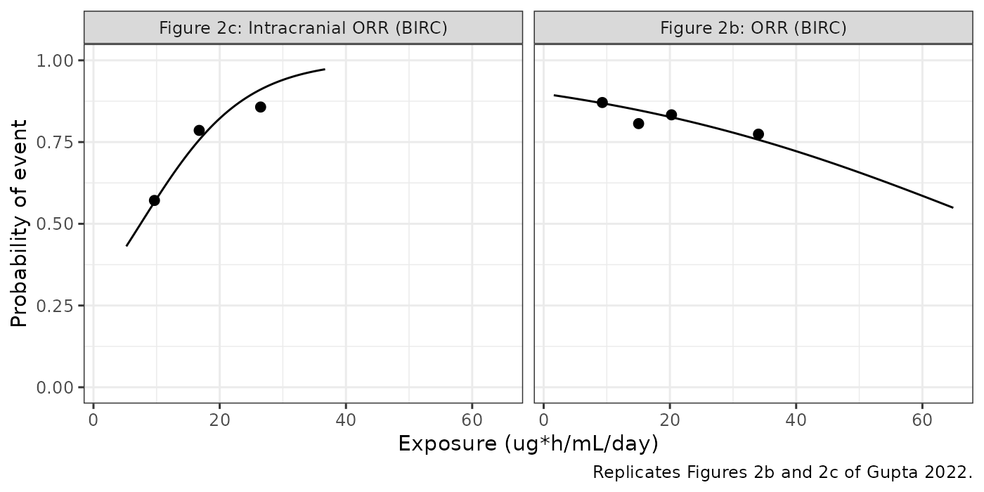
plot_panels(logistic[3:4], "Replicates Figures 3a and 3b of Gupta 2022.")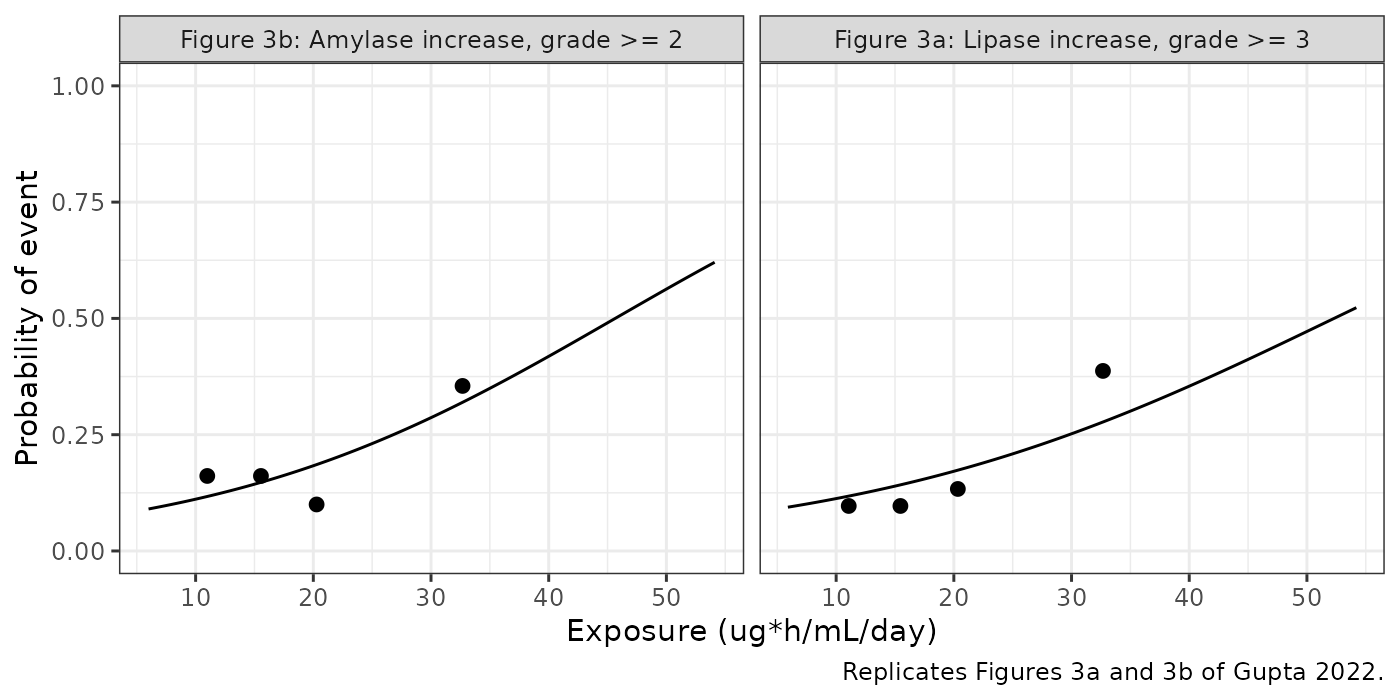
plot_panels(logistic[5:10], "Replicates Supporting Figure S6 of Gupta 2022.")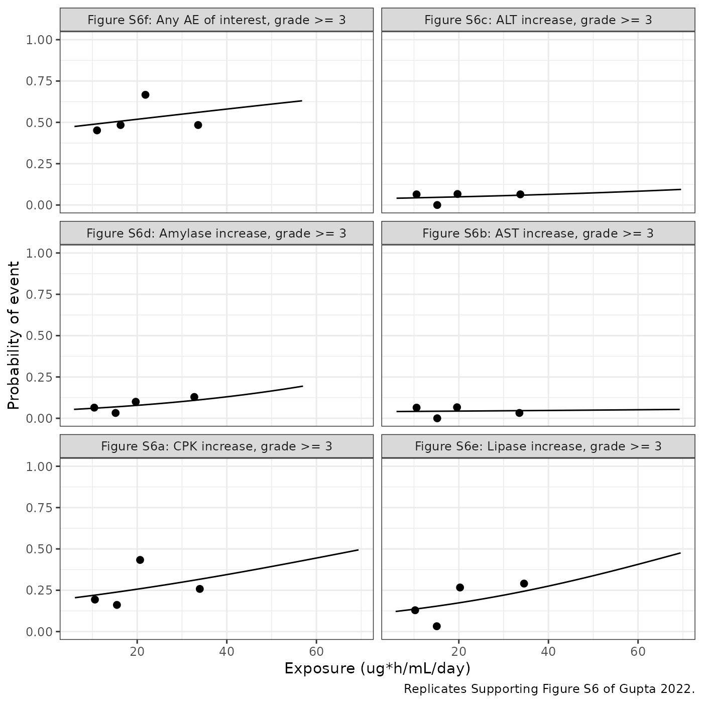
plot_panels(logistic[11:18], "Replicates Supporting Figure S7 of Gupta 2022.")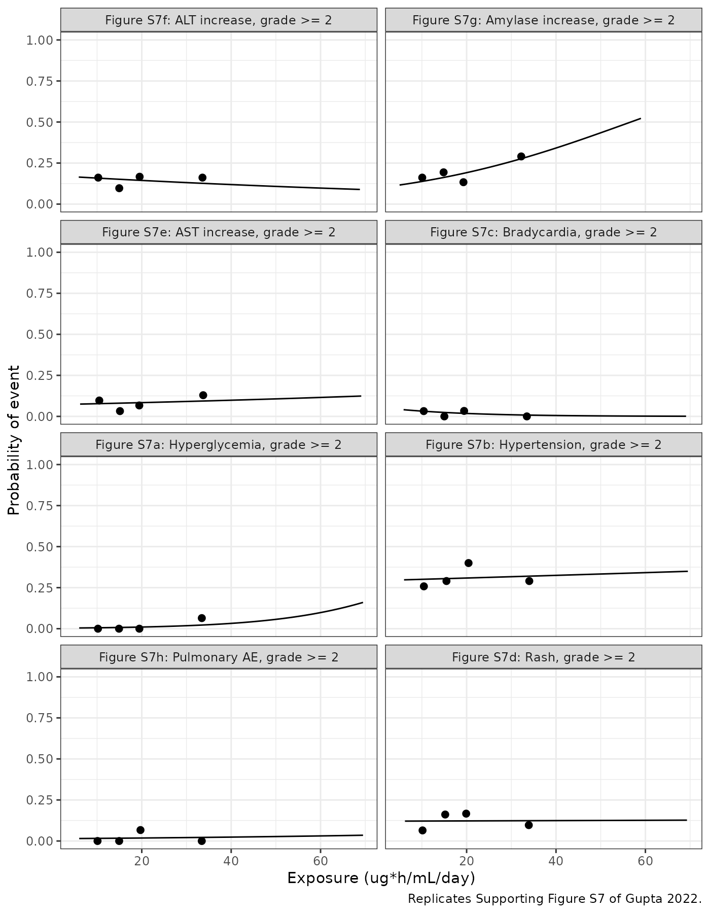
Validation
Event totals
A logistic regression fitted by maximum likelihood with an intercept reproduces the observed number of events exactly: the sum of the fitted probabilities over the patients equals the event count. Evaluating each model at the quartile positions and weighting by the quartile sizes approximates that sum, which checks the figure-derived intercepts against counts the paper prints.
totals <- obs_long |>
  dplyr::rowwise() |>
  dplyr::mutate(p_model = er_eval(mods[[model]], out_col(model), cov_col(model), x)) |>
  dplyr::ungroup() |>
  dplyr::group_by(model) |>
  dplyr::summarise(observed = sum(events), predicted = sum(n * p_model), .groups = "drop") |>
  dplyr::mutate(difference = predicted - observed)
totals |>
  dplyr::rename(
    "Model" = model, "Observed events" = observed,
    "Predicted events" = predicted, "Difference" = difference
  ) |>
knitr::kable(digits = 2, caption = "Observed and model-predicted event totals.")| Model | Observed events | Predicted events | Difference |
|---|---|---|---|
| Gupta_2022_brigatinib_aesi_grade3 | 64 | 64.05 | 0.05 |
| Gupta_2022_brigatinib_alt_grade2 | 18 | 17.86 | -0.14 |
| Gupta_2022_brigatinib_alt_grade3 | 6 | 6.11 | 0.11 |
| Gupta_2022_brigatinib_amylase_grade2 | 24 | 23.50 | -0.50 |
| Gupta_2022_brigatinib_amylase_grade2_d8_14 | 24 | 23.68 | -0.32 |
| Gupta_2022_brigatinib_amylase_grade3 | 10 | 9.73 | -0.27 |
| Gupta_2022_brigatinib_ast_grade2 | 10 | 10.32 | 0.32 |
| Gupta_2022_brigatinib_ast_grade3 | 5 | 5.36 | 0.36 |
| Gupta_2022_brigatinib_bradycardia_grade2 | 2 | 2.53 | 0.53 |
| Gupta_2022_brigatinib_cpk_grade3 | 32 | 31.83 | -0.17 |
| Gupta_2022_brigatinib_hyperglycemia_grade2 | 2 | 1.40 | -0.60 |
| Gupta_2022_brigatinib_hypertension_grade2 | 38 | 37.99 | -0.01 |
| Gupta_2022_brigatinib_iorr | 31 | 31.27 | 0.27 |
| Gupta_2022_brigatinib_lipase_grade3 | 22 | 21.80 | -0.20 |
| Gupta_2022_brigatinib_lipase_grade3_d8_14 | 22 | 21.87 | -0.13 |
| Gupta_2022_brigatinib_orr | 101 | 101.45 | 0.45 |
| Gupta_2022_brigatinib_pulmonary_grade2 | 2 | 2.24 | 0.24 |
| Gupta_2022_brigatinib_rash_grade2 | 15 | 15.05 | 0.05 |
# Table 3 incidences and the Figure 2 response counts.
stopifnot(
  totals$observed[totals$model == "Gupta_2022_brigatinib_orr"] == 101,
  totals$observed[totals$model == "Gupta_2022_brigatinib_iorr"] == 31,
  totals$observed[totals$model == "Gupta_2022_brigatinib_cpk_grade3"] == 32,
  totals$observed[totals$model == "Gupta_2022_brigatinib_aesi_grade3"] == 64,
  totals$observed[totals$model == "Gupta_2022_brigatinib_hypertension_grade2"] == 38,
  # Deterministic: a mis-read intercept moves the predicted total by several
  # events on the larger endpoints.
  all(abs(totals$difference) < 1)
)
Evaluating at the quartile positions rather than at every patient’s exposure is an approximation, so differences of either sign up to about half an event are expected; none reaches one event.
Intracranial response at the steady-state percentiles
Gupta 2022 reports predicted intracranial response probabilities of 0.58, 0.83 and 0.99 at the 5th, 50th and 95th percentiles of steady-state exposure after 180 mg once daily. The 5th and 95th percentiles are 10.1 and 44.6 ug*h/mL; the median is not printed, so it is checked through the exposure at which the model gives 0.83.
p_iorr <- er_eval(mods$Gupta_2022_brigatinib_iorr, "prob_icorr", "AUC_BRIG_SCAN", c(10.1, 44.6))
b_iorr <- coef_of("Gupta_2022_brigatinib_iorr", "e_auc_logit")
a_iorr <- coef_of("Gupta_2022_brigatinib_iorr", "logit_ref")
auc_at_083 <- (qlogis(0.83) - a_iorr) / b_iorr
tibble::tibble(
  Quantity = c("P(iORR) at AUC 10.1", "P(iORR) at AUC 44.6", "AUC giving P(iORR) = 0.83"),
  Model = c(p_iorr, auc_at_083),
  Published = c(0.58, 0.99, NA)
) |>
knitr::kable(digits = 3)| Quantity | Model | Published |
|---|---|---|
| P(iORR) at AUC 10.1 | 0.580 | 0.58 |
| P(iORR) at AUC 44.6 | 0.989 | 0.99 |
| AUC giving P(iORR) = 0.83 | 20.444 | NA |
Cox relative hazards
cox <- c("Gupta_2022_brigatinib_pfs", "Gupta_2022_brigatinib_pfs_scan_tv", "Gupta_2022_brigatinib_pfs_daily_tv")
cox_tab <- dplyr::bind_rows(lapply(cox, function(m) {
  h <- er_eval(mods[[m]], "hr", cov_col(m), c(0, 1, 9.7, 28.3))
  tibble::tibble(
    model = m,
    hr_per_unit = h[2] / h[1],
    hr_q4_vs_q1 = h[4] / h[3]
  )
}))
cox_tab |>
  dplyr::rename(
    "Model" = model, "HR per 1 ug*h/mL/day" = hr_per_unit,
    "HR, 4th vs 1st quartile median" = hr_q4_vs_q1
  ) |>
knitr::kable(digits = 3, caption = "Relative hazards; quartile medians 9.7 and 28.3 ug*h/mL/day from Figure 2a.")| Model | HR per 1 ug*h/mL/day | HR, 4th vs 1st quartile median |
|---|---|---|
| Gupta_2022_brigatinib_pfs | 1.03 | 1.733 |
| Gupta_2022_brigatinib_pfs_scan_tv | 1.02 | 1.445 |
| Gupta_2022_brigatinib_pfs_daily_tv | 1.01 | 1.203 |
Only the static model is significant, and it points the wrong way: a 1.7-fold higher hazard between the first- and fourth-quartile medians. Figure 2a shows the same direction in the Kaplan-Meier curves (hazard ratios against crizotinib of 0.37 in the first and 0.83 in the fourth exposure quartile). Gupta 2022 attributes it to the static metric: patients who stay on treatment longer accumulate dose reductions, so a long PFS is attached to a low last-interval exposure. The two time-varying models, which follow the dose changes, are not significant (p = 0.08 and 0.69).
Assumptions and deviations
Figure-derived coefficients. Gupta 2022 prints no intercept for any of its 18 logistic regressions and no coefficient at all for 12 of them. The intercepts of all 18, and both coefficients of the 12, were read from the fitted curves of Figures 2b, 2c, 3a, 3b, S6 and S7. These are vector graphics in the publisher PDFs, so every node of each curve lies exactly on it and was read without pixel measurement; axes were mapped through the printed tick labels. Where the paper prints an odds ratio, the model uses it and the intercept was refitted with the slope held there. Each model’s annotated panel P value matches the P value in the text wherever both exist (0.108, 0.0486, 0.0389, 0.016, 0.146, 0.0943), so the plotted curves are the reported models and not unadjusted variants.
Two low-incidence panels. In Supporting Figure S7a (hyperglycemia, 2 events) the three curve nodes are not collinear on the logit scale against the tick marks, and the observed-proportion markers of the 0/31 quartiles sit about 0.01 above the drawn zero line, so the panel’s zero is offset; an offset of 0.0074 makes the nodes exactly collinear and was removed. In Supporting Figure S7c (bradycardia, 2 events) the curve flattens onto the zero line above about 40 ug*h/mL/day, where plotting precision is a large relative error, so only the four nodes above a probability of 0.006 were used. Both models rest on 2 events in 123 patients and their coefficients are poorly determined; neither relationship is significant (P = 0.192 and 0.522).
Exposure-only PFS model. In the static PFS analysis
the stepwise covariate search retained ECOG performance status (p <
0.001) and the exposure effect stayed significant, but the paper prints
neither the ECOG coefficient nor the adjusted hazard ratio.
Gupta_2022_brigatinib_pfs encodes the reported
exposure-only hazard ratio and records ECOG in
covariatesDataExcluded.
Not encoded. The static PFS model on time-averaged AUC until progression (“similar exposure-PFS relationships”) prints no hazard ratio. The ORR and iORR models on time-averaged AUC until the best response print an odds ratio (0.97 and 1.09) but no figure, so their intercepts cannot be recovered. Time to first dose reduction was analysed by Kaplan-Meier only. No model file exists for these.
Hazard ratios to two decimals. The three Cox coefficients are the natural logs of hazard ratios printed to two decimals; no standard error or coefficient is printed, so that is the only precision available. No baseline hazard is encoded because a Cox regression does not estimate one.
Deterministic probability outputs. The logistic
models emit a probability with a placeholder additive residual of 0.001,
because rxode2 requires an observation declaration; the source
likelihood is Bernoulli and has no residual. Sample outcomes with
rbinom(n, 1, p).
Typical CL/F versus the first-line post hoc values. The PK model’s typical CL/F at the ALTA-1L median albumin is higher than the geometric mean of the ALTA-1L post hoc estimates (8.45 L/h); Gupta 2022 reports that population predictions slightly under-predicted the first-line data. The exposure-response coefficients were estimated on the post hoc exposures.
Errata
Figure 1 caption units. The Figure 1 caption refers to “baseline albumin of 41 g/dL”; Table 1 and the Results give 41 g/L, which is the physiologically possible value.
Fold-change range in the Results. The Results describe the 5th-95th percentile of post hoc AUC as “-60% to +263%” relative to a typical patient. As fold changes of 0.60 and 2.63 these reproduce the printed 10.1 and 44.6 ug*h/mL from a typical AUC of about 16.9 ug*h/mL (10.1 / 0.60 and 44.6 / 2.63); read as percentage changes they do not. The text most likely meant fold changes of 0.60 and 2.63.