Benznidazole (Frade 2022)
Source:vignettes/articles/Frade_2022_benznidazole.Rmd
Frade_2022_benznidazole.RmdModel and source
- Citation: Frade VP, Moreira CHV, Sabino EC, Bedor DCG, Ghilard FR, Oliveira CDL, Sanches C. Population pharmacokinetic modeling of benznidazole in Brazilian patients with chronic Chagas disease. Rev Inst Med Trop Sao Paulo. 2022;64:e4. doi:10.1590/S1678-9946202264004.
- Description: One-compartment population PK model with first-order absorption and linear elimination for oral benznidazole in Brazilian adults with chronic Chagas disease, fitted to whole-blood (dried blood spot) concentrations with Pmetrics NPAG (Frade 2022; n = 8). Clearance is proportional to body weight normalised to 72.8 kg. Typical values are the means of the non-parametric support-point distributions; IIV is a log-normal approximation of the published CV%.
- Article: https://doi.org/10.1590/S1678-9946202264004 (open access, PMC8815855)
Population
Frade 2022 is a brief communication from a Brazilian prospective cohort of adults with chronic Chagas disease starting standard oral benznidazole (5 mg/kg/day for 60 days) at the Instituto de Infectologia Emilio Ribas and the Hospital das Clinicas (HCFMUSP), Sao Paulo. Eight patients contributed one whole-blood dried blood spot (DBS) sample each on treatment day 15; the cohort was interrupted by the COVID-19 pandemic. Mean age was 50.25 years (SD 6.22; four aged 40-50 and four aged 51-60), 6 of 8 were female, mean weight was 70.16 kg (SD 14.20), and 7 of 8 self-identified as mixed ethnicity and 1 as Black (Table 1 and Results). HIV infection, renal or hepatic impairment, pregnancy and lactation were exclusion criteria.
The same information is available programmatically via
readModelDb("Frade_2022_benznidazole")()$population.
Source trace
| Equation / parameter | Value | Source location |
|---|---|---|
lka |
Ka = 1.66 1/h | Table 2 (mean; SD 0.03, median 1.67, CV 2.0%); Abstract |
lcl |
CL = 6.27 L/h at 72.8 kg | Table 2 (mean; SD 0.09, median 6.32, CV 1.4%); Abstract |
lvc |
V = 38.97 L | Table 2 (mean; SD 8.33, median 37.66, CV 21.4%); Abstract |
e_wt_cl |
1, fixed | Results: “weight normalized to 72.8 kg as a covariate on clearance”; no exponent printed (see Assumptions) |
etalka, etalcl, etalvc
|
log(CV^2 + 1) of 2.0%, 1.4%, 21.4% | Table 2 %CV column |
addSd |
5 mg/L | Methods: “gamma * (1 + 0.1*concentration), value = 5” -> gamma x C0 |
propSd |
0.5 | Methods, same sentence -> gamma x C1 |
d/dt(depot), d/dt(central)
|
one compartment, first-order absorption, linear elimination | Methods (“one compartment structural model … elimination … modeled as a linear process”); Discussion (“open compartment with first-order absorption and elimination”) |
Cc <- central / vc |
whole-blood concentration, mg/L | Methods (DBS whole blood); units from the Figure 1 axis magnitude and the dose-per-volume arithmetic below |
Observed data digitised from Figure 1
Figure 1 (bottom panel) shows every observation against time after dose. The seven visible points were digitised by the maintainers from the published raster image (axis ticks used as calibration). The GOF panels show eight observations; the eighth (6.0 mg/L) is hidden under another point in the VPC panel.
obs_fig1 <- data.frame(
  tad = c(0.83, 1.11, 1.50, 2.49, 3.50, 3.80, 10.41),
  obs = c(10.52, 5.65, 8.22, 6.00, 5.70, 6.00, 1.88)
)
knitr::kable(obs_fig1 |> dplyr::rename("Time after dose (h)" = tad, "Observed (mg/L)" = obs))| Time after dose (h) | Observed (mg/L) |
|---|---|
| 0.83 | 10.52 |
| 1.11 | 5.65 |
| 1.50 | 8.22 |
| 2.49 | 6.00 |
| 3.50 | 5.70 |
| 3.80 | 6.00 |
| 10.41 | 1.88 |
Dosing frequency: the data identify once-daily administration
The paper states a 5 mg/kg/day dose but not whether it was split. The typical-value model at a mean-weight subject (70.16 kg) was solved to steady state under once-daily (5 mg/kg q24h) and twice-daily (2.5 mg/kg q12h) administration and compared with the digitised observations.
mod <- readModelDb("Frade_2022_benznidazole")
mod_typ <- rxode2::zeroRe(mod)
#> ℹ parameter labels from comments will be replaced by 'label()'

wt_mean <- 70.16
ss_profile <- function(dose_mg, tau, wt, tad_grid) {
  n_dose <- 20 * 24 / tau
  ev <- rxode2::et(amt = dose_mg, ii = tau, addl = n_dose - 1, cmt = "depot") |>
    rxode2::et(time = (n_dose - 1) * tau + tad_grid, cmt = "central")
  out <- rxode2::rxSolve(mod_typ, events = ev, params = c(WT = wt),
                         atol = 1e-10, rtol = 1e-10) |> as.data.frame()
  data.frame(tad = out$time - (n_dose - 1) * tau, Cc = out$Cc)
}

pred_qd <- ss_profile(5 * wt_mean, 24, wt_mean, obs_fig1$tad)
#> ℹ omega/sigma items treated as zero: 'etalka', 'etalcl', 'etalvc'
pred_bid <- ss_profile(2.5 * wt_mean, 12, wt_mean, obs_fig1$tad)
#> ℹ omega/sigma items treated as zero: 'etalka', 'etalcl', 'etalvc'

cmp_freq <- obs_fig1 |>
  mutate(
    pred_qd = pred_qd$Cc,
    pred_bid = pred_bid$Cc,
    ratio_qd = pred_qd / obs,
    ratio_bid = pred_bid / obs
  )
knitr::kable(
  cmp_freq |>
    dplyr::rename(
      "Time after dose (h)" = tad, "Observed" = obs,
      "Typical, 5 mg/kg q24h" = pred_qd, "Typical, 2.5 mg/kg q12h" = pred_bid,
      "Ratio q24h" = ratio_qd, "Ratio q12h" = ratio_bid
    ),
  digits = 2,
  caption = "Concentrations in mg/L; ratio = typical prediction / observation."
)| Time after dose (h) | Observed | Typical, 5 mg/kg q24h | Typical, 2.5 mg/kg q12h | Ratio q24h | Ratio q12h |
|---|---|---|---|---|---|
| 0.83 | 10.52 | 6.44 | 3.92 | 0.61 | 0.37 |
| 1.11 | 5.65 | 6.99 | 4.16 | 1.24 | 0.74 |
| 1.50 | 8.22 | 7.24 | 4.25 | 0.88 | 0.52 |
| 2.49 | 6.00 | 6.76 | 3.92 | 1.13 | 0.65 |
| 3.50 | 5.70 | 5.88 | 3.40 | 1.03 | 0.60 |
| 3.80 | 6.00 | 5.63 | 3.25 | 0.94 | 0.54 |
| 10.41 | 1.88 | 2.03 | 1.17 | 1.08 | 0.62 |
stopifnot(
  # Once-daily reproduces the centre of the data and the 10.4 h trough-side
  # sample; twice-daily under-predicts by about 40%.
  abs(median(cmp_freq$ratio_qd) - 1) < 0.15,
  abs(cmp_freq$ratio_qd[cmp_freq$tad > 10] - 1) < 0.15,
  median(cmp_freq$ratio_bid) < 0.75
)
Once-daily dosing centres the typical prediction on the data (median ratio 1.03) and reproduces the 10.4 h sample to within a few percent, while twice-daily dosing under-predicts every sample (median ratio 0.60). The simulations below therefore use 5 mg/kg once daily. The same comparison confirms the concentration units: dose in mg over a volume in litres gives mg/L, on the scale of the unlabelled Figure 1 axis.
Closed-form check
The one-compartment first-order-absorption steady-state profile has a closed form; the solve must agree with it to numerical precision.
cl_typ <- 6.27 * wt_mean / 72.8
kel <- cl_typ / 38.97
ka <- 1.66
dose <- 5 * wt_mean
tad_grid <- seq(0.25, 24, by = 0.25)
closed <- dose * ka / (38.97 * (ka - kel)) *
  (exp(-kel * tad_grid) / (1 - exp(-kel * 24)) - exp(-ka * tad_grid) / (1 - exp(-ka * 24)))
solved <- ss_profile(dose, 24, wt_mean, tad_grid)
#> ℹ omega/sigma items treated as zero: 'etalka', 'etalcl', 'etalvc'
rel_err <- max(abs(solved$Cc - closed) / closed)
rel_err
#> [1] 2.127039e-10
stopifnot(rel_err < 1e-6)
Virtual cohort and VPC (replicates Figure 1, bottom panel)
Weights are drawn from a log-normal distribution with the Table 1 mean and SD; dose is 5 mg/kg once daily for 15 days, observed over the day-15 interval.
set.seed(20220204)
n_sub <- 200
wt_sdlog <- sqrt(log(1 + (14.20 / 70.16)^2))
wt_meanlog <- log(70.16) - wt_sdlog^2 / 2
cohort <- data.frame(id = seq_len(n_sub), WT = rlnorm(n_sub, wt_meanlog, wt_sdlog))

tad_vpc <- seq(0, 24, by = 0.25)
dose_rows <- cohort |>
  tidyr::expand_grid(day = 0:14) |>
  mutate(time = day * 24, amt = 5 * WT, evid = 1L, cmt = "depot") |>
  select(id, time, amt, evid, cmt, WT)
obs_rows <- cohort |>
  tidyr::expand_grid(tad = tad_vpc) |>
  mutate(time = 14 * 24 + tad, amt = NA_real_, evid = 0L, cmt = "central") |>
  select(id, time, amt, evid, cmt, WT)
events <- bind_rows(dose_rows, obs_rows) |> arrange(id, time, desc(evid))

rxode2::rxSetSeed(20220204)
sim <- rxode2::rxSolve(mod, events = events) |>
  as.data.frame() |>
  mutate(tad = time - 14 * 24)
#> ℹ parameter labels from comments will be replaced by 'label()'

vpc <- sim |>
  group_by(tad) |>
  summarise(
    q05 = quantile(Cc, 0.05), q25 = quantile(Cc, 0.25), q50 = median(Cc),
    q75 = quantile(Cc, 0.75), q95 = quantile(Cc, 0.95), .groups = "drop"
  )

ggplot(vpc, aes(tad)) +
  geom_ribbon(aes(ymin = q05, ymax = q95), alpha = 0.2) +
  geom_ribbon(aes(ymin = q25, ymax = q75), alpha = 0.3) +
  geom_line(aes(y = q50)) +
  geom_point(data = obs_fig1, aes(x = tad, y = obs), colour = "blue", shape = 1, size = 2.5) +
  coord_cartesian(xlim = c(0, 12)) +
  labs(
    x = "Time after dose on day 15 (h)",
    y = "Benznidazole whole-blood concentration (mg/L)",
    title = "Replicates Figure 1 (VPC) of Frade 2022",
    caption = "Bands: simulated 5-95% and 25-75%; line: median; circles: observations digitised from Figure 1."
  )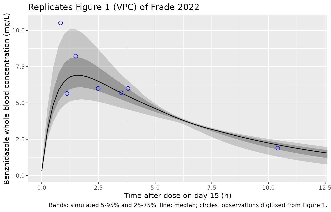
The simulated band is narrower in the absorption phase than the published VPC because the NPAG support-point distribution is summarised here by a log-normal approximation with the very small published CVs for Ka (2.0%) and CL (1.4%); between-subject spread comes mostly from V and body weight.
PKNCA validation
Because both the dose (5 mg/kg) and clearance (proportional to WT /
72.8) scale linearly with weight, the steady-state AUC0-24
is the same for every subject at the typical parameter values:
5 * 72.8 / 6.27 = 58.05 mg*h/L. PKNCA on typical-value
profiles at three body weights checks this identity.
wts <- c(50, 70.16, 90)
tad_nca <- sort(unique(c(seq(0, 2, by = 0.05), seq(2, 24, by = 0.25))))
nca_in <- bind_rows(lapply(wts, function(w) {
  p <- ss_profile(5 * w, 24, w, tad_nca)
  data.frame(id = which(wts == w), treatment = sprintf("%.1f kg", w),
             time = p$tad, Cc = p$Cc, dose = 5 * w)
})) |>
  dplyr::filter(!is.na(Cc))
#> ℹ omega/sigma items treated as zero: 'etalka', 'etalcl', 'etalvc'
#> ℹ omega/sigma items treated as zero: 'etalka', 'etalcl', 'etalvc'
#> ℹ omega/sigma items treated as zero: 'etalka', 'etalcl', 'etalvc'

conc_obj <- PKNCA::PKNCAconc(nca_in, Cc ~ time | treatment + id)
dose_obj <- PKNCA::PKNCAdose(
  nca_in |> distinct(id, treatment, dose) |> mutate(time = 0),
  dose ~ time | treatment + id
)
intervals <- data.frame(start = 0, end = 24, auclast = TRUE, cmax = TRUE, tmax = TRUE, cmin = TRUE)
nca_res <- PKNCA::pk.nca(PKNCA::PKNCAdata(conc_obj, dose_obj, intervals = intervals))

nca_tbl <- as.data.frame(nca_res$result) |>
  select(treatment, PPTESTCD, PPORRES) |>
  tidyr::pivot_wider(names_from = PPTESTCD, values_from = PPORRES)
knitr::kable(
  nca_tbl |>
    dplyr::rename("Body weight" = treatment, "AUC0-24" = auclast, "Cmax" = cmax, "Tmax" = tmax, "Cmin" = cmin),
  digits = 2,
  caption = "Typical-value steady-state NCA, 5 mg/kg once daily (mg/L, h, mg*h/L)."
)| Body weight | AUC0-24 | Cmax | Cmin | Tmax |
|---|---|---|---|---|
| 50.0 kg | 58.05 | 5.72 | 0.52 | 1.70 |
| 70.2 kg | 58.05 | 7.24 | 0.25 | 1.55 |
| 90.0 kg | 58.05 | 8.73 | 0.11 | 1.45 |
Frade 2022 reports no NCA table, so there is no published Cmax / AUC
to compare against; the digitised Figure 1 observations above are the
only published exposure data. As a further consistency check, the
largest population prediction in the Figure 1
observed-versus-population-predicted panel is about 8.65 mg/L, close to
the typical Cmax of a 90 kg subject above (roughly one SD
above the mean weight).
Assumptions and deviations
-
Weight covariate form. The Results say only that
“weight normalized to 72.8 kg” was included as a covariate on clearance,
and Table 2 lists no covariate coefficient. The Pmetrics “normalized to”
idiom is read as the linear ratio
CL = CL_pop * WT / 72.8(exponent fixed at 1, carried ase_wt_cl). A fixed allometric 0.75 would change clearance by up to 10% across 50-90 kg. 72.8 kg is not the reported mean weight (70.16 kg) and is presumably the cohort median. - Dosing frequency. The paper gives 5 mg/kg/day without a dosing interval. Once-daily administration is inferred from the digitised Figure 1 data (see above), where the twice-daily alternative under-predicts every observation, by about 40% at the median.
-
Non-parametric estimates. Pmetrics NPAG estimates a
discrete support-point distribution. The Table 2 means are used as
typical values and the %CV column as a log-normal IIV approximation,
omega^2 = log(CV^2 + 1); the median column (Ka 1.67, CL 6.32, V 37.66) differs by less than 4%. With one sample from each of eight patients these CVs mostly measure how precisely the parameters were estimated, and should not be read as well-characterised between-subject variability. -
Residual error. The Methods give the Pmetrics error
model as
gamma * (1 + 0.1 * concentration)with “value = 5”. This is encoded asaddSd = 5 * 1 = 5mg/L andpropSd = 5 * 0.1 = 0.5. The sentence does not say whether 5 is the converged gamma or its starting value, and the result is large relative to the 2-10 mg/L observations, so simulations that add residual error should be interpreted with caution. The VPC above shows the model prediction without residual error, asCc. -
Matrix. Concentrations are in whole blood (dried
blood spots), not plasma, so the parameters are not directly comparable
with the plasma models of Soy 2015 (
Soy_2015_benznidazole) or Altcheh 2023. - Apparent parameters. Bioavailability was not estimated; CL and V are apparent oral values.
- Virtual cohort. Only weight is simulated; no weight range was reported, so the log-normal weight distribution is not truncated.