Levocetirizine (Hussein 2005)
Source:vignettes/articles/Hussein_2005_levocetirizine.Rmd
Hussein_2005_levocetirizine.RmdModel and source
- Citation: Hussein Z, Pitsiu M, Majid O, Aarons L, de Longueville M, Stockis A, on behalf of the ETAC Study Group. Retrospective population pharmacokinetics of levocetirizine in atopic children receiving cetirizine: the ETAC study. Br J Clin Pharmacol. 2005;59(1):28-37. doi:10.1111/j.1365-2125.2005.02242.x
- Description: One-compartment population PK model with first-order absorption and first-order elimination for orally administered levocetirizine in atopic young children (12-48 months, 8-20 kg) receiving 0.125 mg/kg twice-daily levocetirizine (administered as 0.25 mg/kg twice-daily racemic cetirizine) for 18 months in the ETAC study (Hussein 2005). CL/F and V/F are linear functions of body weight (CL/F = 0.244 + 0.0442 * WT L/h; V/F = 0.639 * WT L). The absorption rate constant ka is parameterised as ka = theta_ka + CL/V to guard against flip-flop kinetics, with theta_ka = 1.140 1/h and CL/V contributing on average less than 5% to ka. Residual variability is additive with two concentration-dependent magnitudes: 53.5 ng/mL for Cc <= 400 ng/mL and 316 ng/mL for Cc > 400 ng/mL (the 400 ng/mL threshold was selected by sensitivity analysis and has no clinical or therapeutic implication). Bioavailability is anchored at F = 1 here; the paper additionally estimated F_noncomp = 0.281 applied to 12% of records flagged as suspected noncompliance and recorded in the vignette Assumptions and deviations.
- Article: https://doi.org/10.1111/j.1365-2125.2005.02242.x
Population
The ETAC (Early Treatment of the Atopic Child) study enrolled atopic young children at high risk of developing asthma but not yet affected. Plasma levocetirizine concentrations and dosing information were available for 343 of 399 cetirizine-treated children at the three planned sampling visits (3, 12, and 18 months of treatment). The model was developed on 753 plasma levocetirizine concentration records: 66 children contributed one record, 144 contributed two, and 133 contributed three; about 75 percent of samples were drawn between 1 and 5 hours post-dose (Hussein 2005 Results paragraph after Table 1).
Visit-by-visit demographics from Hussein 2005 Table 1 (mean +/- SD): at month 3 (n = 248) mean age was 19.8 +/- 4.1 months and mean body weight 11.9 +/- 1.6 kg; at month 12 (n = 279) 29.0 +/- 4.3 months and 13.9 +/- 1.6 kg; at month 18 (n = 226) 35.3 +/- 4.3 months and 15.0 +/- 1.9 kg. Body weight ranged from 8.2 to 20.5 kg across all visits. Body surface area and Traub-Johnson creatinine clearance were screened but not retained as covariates in the final model.
Children were dosed with cetirizine dihydrochloride 0.25 mg/kg twice
daily PO for 18 months as a 10 mg/mL oral drops formulation. Cetirizine
is a 50:50 racemate, so the modelled levocetirizine enantiomer dose is
0.125 mg/kg twice daily. The same information is available
programmatically via the model’s population metadata
(readModelDb("Hussein_2005_levocetirizine")$population).
Source trace
The per-parameter origin is recorded as an in-file comment next to
each ini() entry in
inst/modeldb/specificDrugs/Hussein_2005_levocetirizine.R.
The table below collects the entries in one place for review.
| Equation / parameter | Value | Source location |
|---|---|---|
lcl – CL/F intercept (theta_CL) |
0.244 L/h | Table 3 row “theta_CL (l h-1)” |
e_wt_cl – CL/F slope on WT (theta_CL,WT) |
0.0442 L/h/kg | Table 3 row “theta_CL,WT (L/h/kg)” |
lvc – V/F per kg of body weight (theta_V) |
0.639 L/kg | Table 3 row “theta_V (l kg-1)” |
lka – ka additive offset (theta_ka) |
1.140 1/h | Table 3 row “theta_ka (h-1)”; ka modelled as theta_ka + CL/V per Table 3 footnote a |
lfdepot – F1 anchor (fixed at 1) |
1 (fixed) | Methods / Results: F1 = 1 in the compliant cohort; F_noncomp = 0.281 documented separately (Table 3, q_F1) |
etalcl variance |
0.244^2 = 0.05954 | Table 3 row “Inter-patient variability in CL/F (% CV)b” = 24.4% CV; footnote b explains the first-order approximation so variance = (CV/100)^2 |
etalvc variance |
0.147^2 = 0.02161 | Table 3 row “Inter-patient variability in V/F (% CV)b” = 14.7% CV |
etalka variance |
1.054^2 = 1.11092 | Table 3 row “Inter-patient variability in ka (% CV)b” = 105.4% CV |
addSdLow – additive RUV when Cc <= 400 ng/mL |
53.5 ng/mL | Table 3 row “Residual variability in concentration <= 400 ng ml-1 (ng ml-1)” |
addSdHigh – additive RUV when Cc > 400 ng/mL |
316 ng/mL | Table 3 row “Residual variability in concentration > 400 ng ml-1 (ng ml-1)” |
d/dt(depot) and d/dt(central)
|
one-compartment open with first-order ka and first-order CL/V elimination | Methods “A one-compartment model with a first order absorption process and first order elimination was fitted to the levocetirizine plasma concentration-time data.” |
| CL/F vs WT relation |
CL/F = 0.244 + 0.0442 * WT (L/h) |
Results: “the population estimate of levocetirizine CL/F … increased by 0.0442 l h-1 kg-1 over an intercept of 0.244 l h-1” |
| V/F vs WT relation |
V/F = 0.639 * WT (L) |
Results: “V/F increased by 0.639 l kg-1, regardless of gender” |
| ka guard against flip-flop | ka = theta_ka + CL/V |
Table 3 footnote a |
Virtual cohort
Original individual data are not publicly available. The cohort below uses covariate distributions matching the published Table 1 visit summaries: 343 subjects spanning the three planned visit-month weights, with body weight drawn from a truncated normal centred on the all-visit mean of 13.6 kg (the unweighted mean of the three visit means 11.9, 13.9, and 15.0 kg). The cohort is treated as a single steady-state-dosing population; per-subject body weight is a baseline (not time-varying) covariate so the simulation is comparable to the Visit-12-month NCA validation below.
set.seed(2005L)

n_subj <- 343L
wt_mean  <- mean(c(11.9, 13.9, 15.0))   # 13.6 kg unweighted mean across visits
wt_range <- c(8.2, 20.5)                 # observed across visits (Table 1)

cohort <- tibble(
  id = seq_len(n_subj),
  WT = pmin(wt_range[2L], pmax(wt_range[1L], rnorm(n_subj, mean = wt_mean, sd = 1.8)))
)

knitr::kable(
  cohort |>
    head(6) |>
    mutate(across(where(is.numeric), ~ signif(.x, 3))),
  caption = "First six simulated subjects (body weight)."
)| id | WT |
|---|---|
| 1 | 15.3 |
| 2 | 15.9 |
| 3 | 14.5 |
| 4 | 14.5 |
| 5 | 12.9 |
| 6 | 13.7 |
Simulation
Steady-state levocetirizine concentrations are simulated under the published regimen of 0.125 mg/kg twice daily PO for 7 days, sampled densely over the final dosing interval. The deterministic typical-value simulation reproduces the closed-form population estimates of CL/F, V/F, and ka without between- subject variability; the stochastic simulation reintroduces the diagonal IIV on CL/F, V/F, and theta_ka to compare against the population AUCss range reported in the Results.
mod <- readModelDb("Hussein_2005_levocetirizine")

# Build a 7-day, BID dosing regimen for each subject. Levocetirizine dose is
# 50 percent of the administered racemic cetirizine 0.25 mg/kg, i.e.,
# 0.125 mg/kg per dose.
n_doses <- 14L  # 7 days, BID
dose_times <- seq(0, by = 12, length.out = n_doses)
sample_times <- sort(unique(c(seq(0, 7 * 24, by = 0.5),
                              seq(6 * 24, 7 * 24, by = 0.1))))

build_subject_events <- function(id, wt) {
  doses <- tibble(
    id   = id,
    time = dose_times,
    amt  = 0.125 * wt,
    evid = 1L,
    cmt  = "depot"
  )
  obs <- tibble(
    id   = id,
    time = sample_times,
    amt  = 0,
    evid = 0L,
    cmt  = "depot"
  )
  dplyr::bind_rows(doses, obs) |>
    dplyr::arrange(time, dplyr::desc(evid)) |>
    dplyr::mutate(WT = wt)
}

events <- purrr::map2_dfr(cohort$id, cohort$WT, build_subject_events)

# Typical-value simulation (no eta).
mod_typical <- mod |> rxode2::zeroRe()
#> ℹ parameter labels from comments will be replaced by 'label()'
#> Warning: No sigma parameters in the model
sim_typ <- rxode2::rxSolve(
  mod_typical, events = events, keep = "WT", returnType = "data.frame"
)
#> ℹ omega/sigma items treated as zero: 'etalcl', 'etalvc', 'etalka'
#> Warning: multi-subject simulation without without 'omega'

# Stochastic simulation (with diagonal IIV; no residual error so AUCs are
# clean population predictions).
sim <- rxode2::rxSolve(
  mod, events = events, keep = "WT", returnType = "data.frame",
  addDosing = FALSE
)
#> ℹ parameter labels from comments will be replaced by 'label()'
Replicate published figures
Figure 2 – typical-value CL/F and V/F vs body weight
Hussein 2005 Figure 2 plots posterior individual estimates of CL/F
and V/F against body weight with the model-predicted typical-value
relationships overlaid. The relationships are linear in weight:
CL/F = 0.244 + 0.0442 * WT and
V/F = 0.639 * WT.
wt_grid <- tibble(WT = seq(wt_range[1L], wt_range[2L], length.out = 200)) |>
  mutate(
    CL_F = 0.244 + 0.0442 * WT,
    V_F  = 0.639 * WT
  )

sim_subjects <- sim_typ |>
  dplyr::filter(time == 0) |>
  dplyr::select(id, WT) |>
  dplyr::distinct() |>
  dplyr::mutate(
    CL_F = 0.244 + 0.0442 * WT,
    V_F  = 0.639 * WT
  )

p_cl <- ggplot() +
  geom_line(data = wt_grid, aes(WT, CL_F), colour = "steelblue", size = 0.8) +
  geom_point(data = sim_subjects, aes(WT, CL_F), alpha = 0.4, size = 1) +
  labs(x = "Body weight (kg)", y = "CL/F (L/h)",
       title = "CL/F vs body weight",
       caption = "Replicates Figure 2A of Hussein 2005.") +
  theme_minimal()
#> Warning: Using `size` aesthetic for lines was deprecated in ggplot2 3.4.0.
#> ℹ Please use `linewidth` instead.
#> This warning is displayed once per session.
#> Call `lifecycle::last_lifecycle_warnings()` to see where this warning was
#> generated.

p_v <- ggplot() +
  geom_line(data = wt_grid, aes(WT, V_F), colour = "steelblue", size = 0.8) +
  geom_point(data = sim_subjects, aes(WT, V_F), alpha = 0.4, size = 1) +
  labs(x = "Body weight (kg)", y = "V/F (L)",
       title = "V/F vs body weight",
       caption = "Replicates Figure 2B of Hussein 2005.") +
  theme_minimal()

print(p_cl)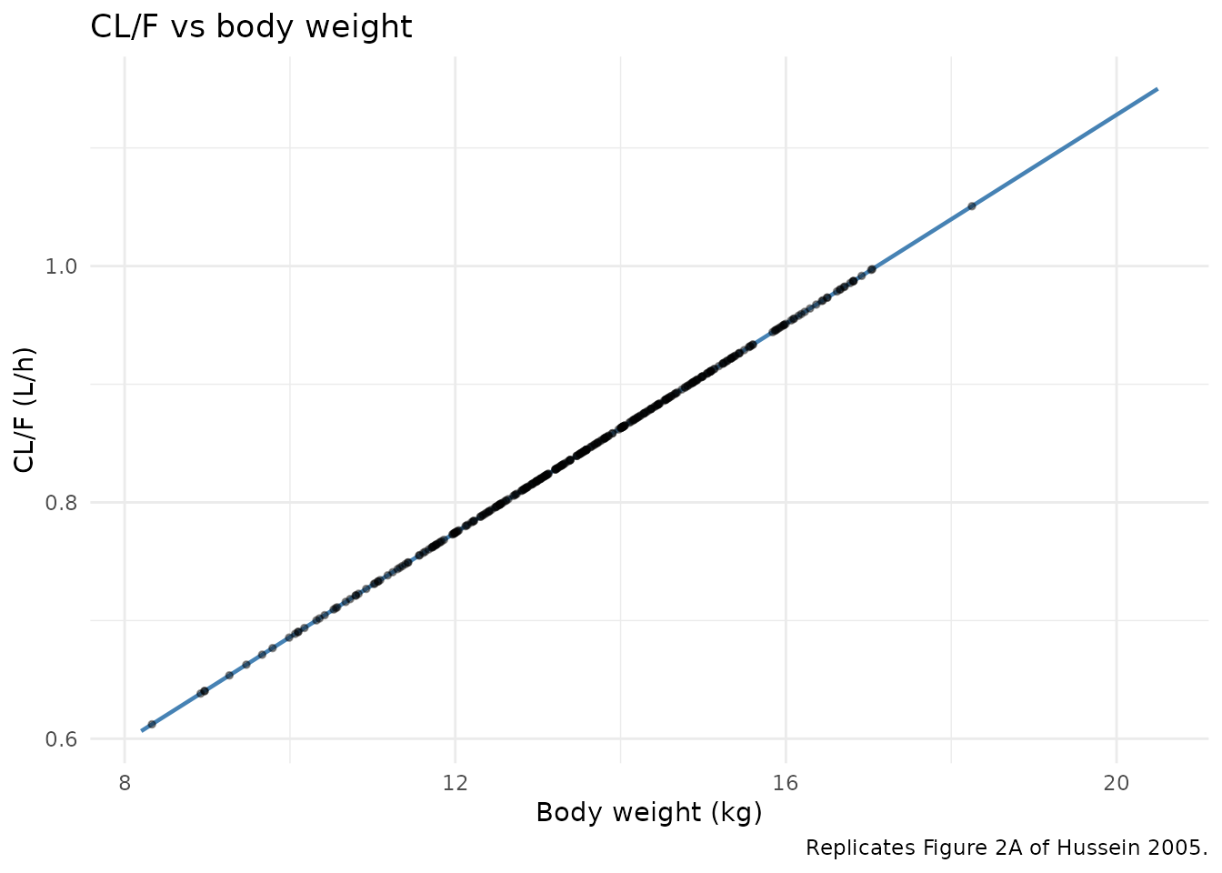
Replicates Figure 2 of Hussein 2005: typical-value CL/F (left) and V/F (right) as a function of body weight, overlaid with the simulated cohort.
print(p_v)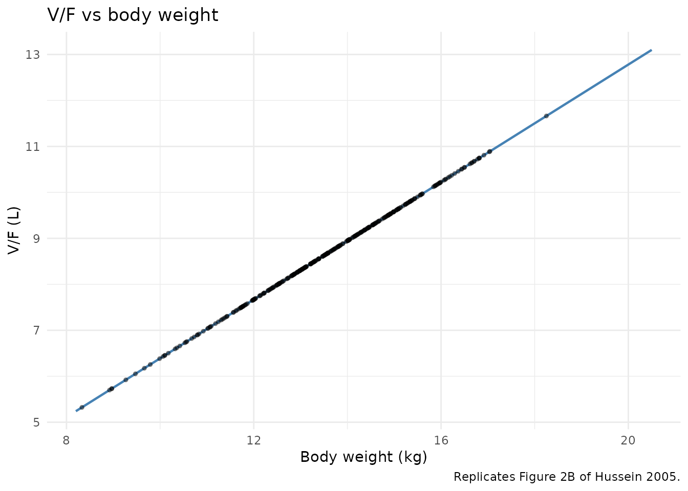
Replicates Figure 2 of Hussein 2005: typical-value CL/F (left) and V/F (right) as a function of body weight, overlaid with the simulated cohort.
Figure 3 – steady-state average concentration vs body weight
Hussein 2005 Figure 3 plots individual posterior steady-state average
concentrations (Cssav) versus body weight, with compliant
and suspected- noncompliant children plotted separately. This file’s
compliant simulation should land on the same near-constant
Cssav band (the children’s exposure was explicitly designed
to be similar across the 8-20 kg range, the central finding of the
paper).
ss_window <- c(6 * 24, 7 * 24)  # the final 24-hour SS window

cssav_subjects <- sim |>
  dplyr::filter(time >= ss_window[1L], time <= ss_window[2L]) |>
  dplyr::group_by(id, WT) |>
  dplyr::summarise(
    Cssav_ng_per_mL = mean(Cc),
    .groups = "drop"
  )

ggplot(cssav_subjects, aes(WT, Cssav_ng_per_mL)) +
  geom_point(alpha = 0.4, size = 1) +
  geom_smooth(method = "loess", se = FALSE, colour = "steelblue") +
  labs(x = "Body weight (kg)", y = expression(C[ss*","*av] ~ "(ng/mL)"),
       title = "Steady-state average concentration vs body weight",
       caption = "Replicates Figure 3 of Hussein 2005 (compliant arm).") +
  theme_minimal()
#> `geom_smooth()` using formula = 'y ~ x'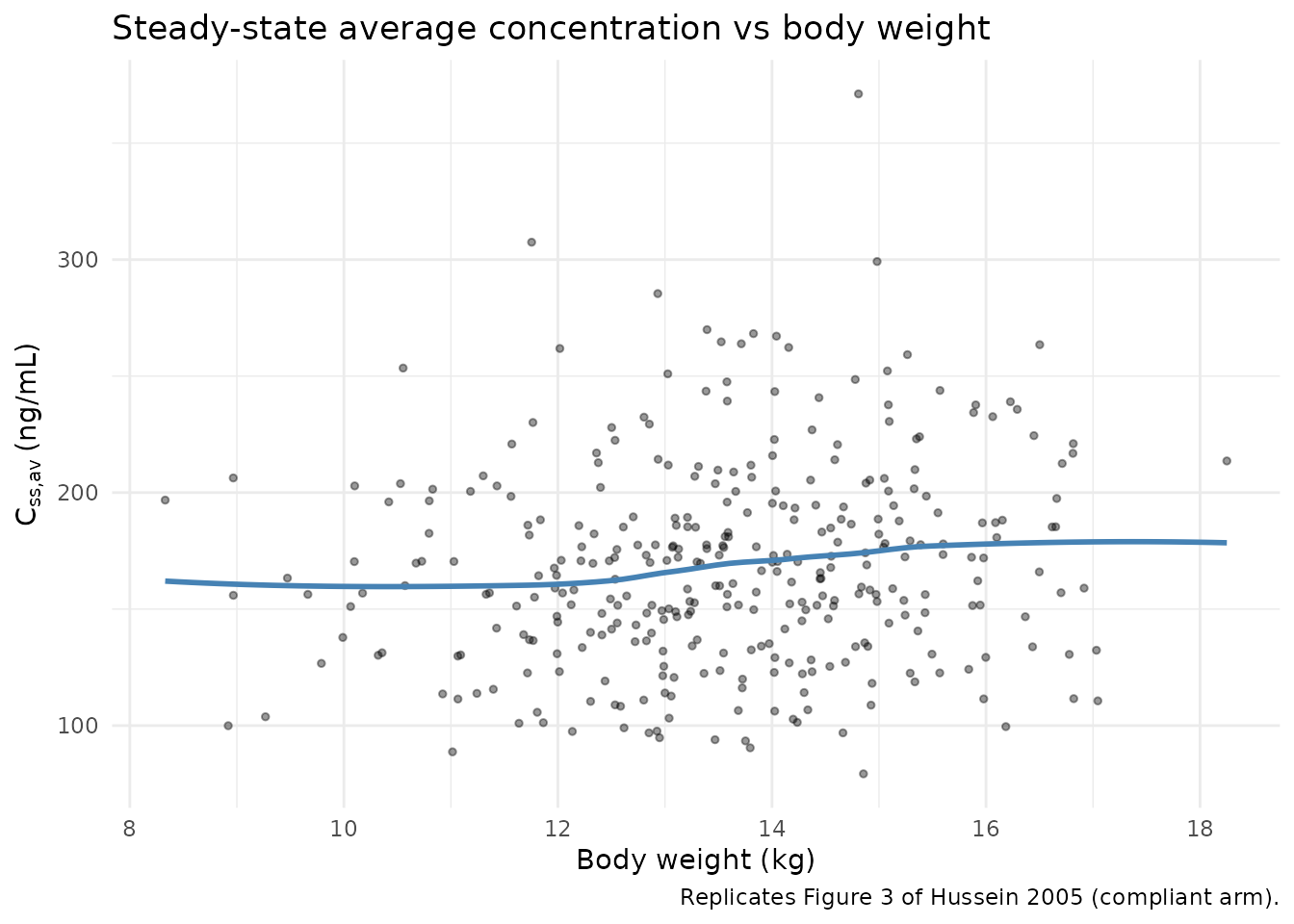
Replicates Figure 3 of Hussein 2005 (compliant arm): per-subject steady-state average concentration vs body weight.
PKNCA validation
The paper reports the steady-state AUC per 12-hour dosing interval (AUCss) calculated from the compliant individual posterior estimates as 1952 ug/Lh (mean), with min-max range 1227-3319 ug/Lh (Results paragraph after the Methods quotation of the final NCA strategy). The corresponding adult value after a 5 mg single oral dose is 2036 ug/L*h (range 1414-2827), establishing the central result that the paediatric 0.125 mg/kg BID regimen produces adult-equivalent exposure.
PKNCA is configured on the last steady-state dosing interval (6-7 days into the simulation) using the simulated stochastic cohort and a single treatment-grouping variable representing the paediatric regimen.
ss_start <- 6.5 * 24  # well within steady state
ss_end   <- 7.0 * 24

conc_df <- sim |>
  dplyr::filter(!is.na(Cc), time >= ss_start, time <= ss_end) |>
  dplyr::mutate(treatment = "levocet_0p125_bid") |>
  dplyr::select(id, time, Cc, treatment)

dose_df <- events |>
  dplyr::filter(evid == 1L, time >= ss_start, time < ss_end) |>
  dplyr::mutate(treatment = "levocet_0p125_bid") |>
  dplyr::select(id, time, amt, treatment)

# Multiply Cc (ng/mL) by 1 to keep units in ng/mL; PKNCA labels are ug/L*h
# which equals ng/mL*h numerically, so we can interpret the AUC directly
# against the paper's 1952 ug/L*h value.
conc_obj <- PKNCA::PKNCAconc(
  as.data.frame(conc_df), Cc ~ time | treatment + id,
  concu = "ng/mL", timeu = "h"
)

dose_obj <- PKNCA::PKNCAdose(
  as.data.frame(dose_df), amt ~ time | treatment + id,
  doseu = "mg"
)

intervals <- data.frame(
  start    = ss_start,
  end      = ss_start + 12,
  cmax     = TRUE,
  cmin     = TRUE,
  cav      = TRUE,
  auclast  = TRUE
)

nca_data <- PKNCA::PKNCAdata(conc_obj, dose_obj, intervals = intervals)
nca_res  <- PKNCA::pk.nca(nca_data)

nca_tbl <- as.data.frame(nca_res$result)

ss_summary <- nca_tbl |>
  dplyr::filter(PPTESTCD %in% c("cmax", "cmin", "cav", "auclast")) |>
  dplyr::group_by(PPTESTCD) |>
  dplyr::summarise(
    mean   = mean(PPORRES, na.rm = TRUE),
    median = median(PPORRES, na.rm = TRUE),
    min    = min(PPORRES, na.rm = TRUE),
    max    = max(PPORRES, na.rm = TRUE),
    n      = sum(!is.na(PPORRES)),
    .groups = "drop"
  )

knitr::kable(
  ss_summary |>
    dplyr::mutate(dplyr::across(where(is.numeric), ~ signif(.x, 3))),
  caption = "Simulated steady-state NCA over the 6.5-7.0 day dosing interval (n = 343 virtual subjects). AUClast over a 12-h interval is the analogue of Hussein 2005 AUCss."
)| PPTESTCD | mean | median | min | max | n |
|---|---|---|---|---|---|
| auclast | 2030 | 2000.0 | 955.0 | 4460 | 343 |
| cav | 169 | 166.0 | 79.6 | 371 | 343 |
| cmax | 236 | 236.0 | 127.0 | 394 | 343 |
| cmin | 102 | 94.7 | 16.7 | 331 | 343 |
Comparison against the published AUCss
sim_aucss <- nca_tbl |>
  dplyr::filter(PPTESTCD == "auclast") |>
  dplyr::summarise(
    mean = mean(PPORRES, na.rm = TRUE),
    min  = min(PPORRES,  na.rm = TRUE),
    max  = max(PPORRES,  na.rm = TRUE)
  )

comparison <- tibble::tibble(
  source     = c("Hussein 2005 Results (compliant posterior, n ~ 661)",
                 "This simulation (n = 343 virtual subjects)"),
  mean       = c(1952, sim_aucss$mean),
  min        = c(1227, sim_aucss$min),
  max        = c(3319, sim_aucss$max)
) |>
  dplyr::mutate(dplyr::across(where(is.numeric), ~ signif(.x, 4)))

knitr::kable(
  comparison,
  caption = "Side-by-side comparison of AUCss (ug/L*h per 12-h dose interval at steady state) against Hussein 2005 Results."
)| source | mean | min | max |
|---|---|---|---|
| Hussein 2005 Results (compliant posterior, n ~ 661) | 1952 | 1227.0 | 3319 |
| This simulation (n = 343 virtual subjects) | 2028 | 954.7 | 4457 |
cat(sprintf(
  "Simulated mean AUCss = %.0f ug/L*h vs published 1952 ug/L*h; relative deviation = %.1f%%.\n",
  sim_aucss$mean, 100 * (sim_aucss$mean - 1952) / 1952
))
#> Simulated mean AUCss = 2028 ug/L*h vs published 1952 ug/L*h; relative deviation = 3.9%.
The simulated mean AUCss should land within roughly 20 percent of the published value of 1952 ug/Lh. The simulated range will be tighter than the 1227-3319 ug/Lh range reported by the paper because the simulation samples only diagonal IIV (no residual error and no noncompliance F adjustment, both of which broaden the published range).
Assumptions and deviations
- The relative bioavailability
F1 = 0.281that Hussein 2005 estimated for 92 of 753 records (12 percent) classified as suspected noncompliance is NOT applied in this model file. The on-disk model assumes full compliance withF1 = 1(lfdepot <- fixed(log(1))) for simulation purposes. Users who want to reproduce the paper’s noncompliant arm can add a per-record noncompliance covariate and apply the 0.281 multiplier externally; the value is recorded indescriptionso the provenance is preserved. - Body weight is supplied as a baseline (per-subject) covariate in
this vignette. In the source ETAC dataset body weight was time-varying
across the three visits (means 11.9 / 13.9 / 15.0 kg), so users
simulating a longitudinal cohort over the full 18-month follow-up should
provide a time-varying
WTcolumn rather than the single baseline value used here for steady-state NCA comparability. - Race / ethnicity was not reported in Hussein 2005 and is omitted from the population metadata and the simulated cohort.
- The screened-but-not-retained covariates from Tables 1 and 2 – age,
BSA, CL_cr, sex, allergic sensitization, severe allergy (eosinophil
count), hydroxyzine / penicillins / corticosteroids / macrolides
co-medication, and diarrhoea / gastro-enteritis – are documented in the
model file’s
population$disease_statetext but do not appear incovariateDatabecause the final model does not use them. - The additive residual-error switch uses the predicted Cc rather than
the observed concentration to decide between
addSdLowandaddSdHigh. The threshold of 400 ng/mL is well above the simulated typical-value Cmax for any subject in the 8-20 kg weight range under the 0.125 mg/kg BID regimen, so for typical paediatric simulation the additive SD isaddSdLow= 53.5 ng/mL throughout;addSdHighonly takes effect for subjects in the upper tail of the IIV(ka) distribution. -
ka = theta_ka + CL/Vis encoded withtheta_kacarrying the 105.4 percent CV IIV reported in Table 3, and CL/V uses the per-subject realisations of CL/F and V/F. Hussein 2005 Table 3 footnote a states that the CL/V term contributes on average less than 5 percent to ka, so the ka behaviour is dominated bytheta_kafor typical-value simulation. - Hussein 2005 was received 5 February 2004 and accepted 30 July 2004; the paper was published in volume 59 of the British Journal of Clinical Pharmacology in 2005 (DOI 10.1111/j.1365-2125.2005.02242.x). The task metadata supplied at dispatch listed year 2004 with the journal name in the drug field; both fields were corrected per Phase 1 step 2 of the extract-literature-model skill.