Moxifloxacin in post-bariatric surgery patients (Colin 2014)
Source:vignettes/articles/Colin_2014_moxifloxacin.Rmd
Colin_2014_moxifloxacin.RmdModel and source
- Citation: Colin P, Eleveld DJ, Struys MMRF, T’Jollyn H, Van Bortel LM, Ruige J, De Waele J, Van Bocxlaer J, Boussery K. Moxifloxacin dosing in post-bariatric surgery patients. Br J Clin Pharmacol. 2014 Jul;78(1):84-90. doi:10.1111/bcp.12302. PMID 24330006; PMCID PMC4168384.
- Description: Three-compartment population PK model for moxifloxacin in post-bariatric (roux-en-y gastric bypass) volunteers (Colin 2014): linear first-order absorption (no lag, no transit) into a central compartment with two peripheral compartments, allometric scaling on lean body mass (exponent 0.75 on all CL terms and 1 on all volumes, reference LBM 60 kg), and inter-individual variability on ka, central volume, and clearance. Single 400 mg oral and 400 mg 1-h IV infusion doses are fit simultaneously with an implicit bioavailability of 1.
- Article: https://doi.org/10.1111/bcp.12302
Population
Colin et al. (2014) developed the population pharmacokinetic model from a single-centre randomised crossover trial of 12 volunteers (4 men, 8 women) who had undergone roux-en-y gastric bypass at least 6 months prior to enrolment (De Smet et al. 2012). Baseline demographics from Colin 2014 Table 1 (median [range]): age 41 [25-57] years; total body weight 78.1 [57.4-104.0] kg; lean body mass 51.7 [41.9-77.6] kg (James equation); height 1.68 [1.58-1.99] m; serum albumin 3.96 [3.54-4.40] g/dL; Cockroft-Gault creatinine clearance 131.9 [100.4-221.5] mL/min. Subjects were generally in good condition and were not actively infected. Each volunteer received two single 400 mg moxifloxacin doses, separated by a 1-week washout: once as a tablet (oral) and once as a 1-h intravenous infusion. Total observed plasma concentrations were 432 (paired oral + IV profiles spanning 0 to 72 h post-dose; HPLC-fluorescence assay, De Smet et al. 2009).
The same information is available programmatically via
readModelDb("Colin_2014_moxifloxacin")$population.
Source trace
Per-parameter origin comments are recorded in
inst/modeldb/specificDrugs/Colin_2014_moxifloxacin.R. The
table below collects them in one place. All point estimates are from
Colin 2014 Table 2 for a typical subject with LBM = 60 kg.
| Equation / parameter | Value | Source location |
|---|---|---|
lka (absorption rate constant ka) |
log(0.95) | Table 2 ka = 0.95 1/h [95% boot 0.72, 1.21]; only structural parameter without LBM scaling |
lcl (clearance CL at LBM = 60 kg) |
log(8.60) | Table 2 CL * (LBM/60)^0.75 = 8.60 L/h [95% boot 7.80, 9.70] |
lvc (central volume V1 at LBM = 60 kg) |
log(47.7) | Table 2 V1 * (LBM/60) = 47.7 L [95% boot 31.6, 78.6] |
lq (Q2 at LBM = 60 kg) |
log(105.3) | Table 2 Q2 * (LBM/60)^0.75 = 105.3 L/h [95% boot 55.2, 140.0] |
lvp (V2 at LBM = 60 kg) |
log(61.5) | Table 2 V2 * (LBM/60) = 61.5 L [95% boot 37.6, 75.7] |
lq2 (Q3 at LBM = 60 kg) |
log(1.35) | Table 2 Q3 * (LBM/60)^0.75 = 1.35 L/h [95% boot 1.23, 1.56] |
lvp2(V3 at LBM = 60 kg) |
log(48.4) | Table 2 V3 * (LBM/60) = 48.4 L [95% boot 34.4, 92.9] |
allo_cl (allometric exponent on CL terms) |
fixed(0.75) | Discussion: removing the 0.75 exponent gave dAICc = -0.50 (no improvement); kept fixed |
allo_v (allometric exponent on V terms) |
fixed(1.00) | Table 2 footnote: volumes scale linearly with LBM/60 |
etalka (variance) |
0.24 | Table 2 omega^2(ka) = 0.24 |
etalvc (variance) |
0.14 | Table 2 omega^2(V1) = 0.14 |
etalcl (variance) |
0.04 | Table 2 omega^2(CL) = 0.04 |
propSd |
sqrt(0.03) = 0.1732 | Table 2 sigma^2(Proportional) = 0.03 |
| Three-compartment ODE with first-order absorption | structural | Methods and Figure 2 (final model schematic); no lag, no transit |
Virtual cohort
The original observed dataset is not publicly available. We simulate two virtual cohorts patterned on Colin 2014 Figure 7, which compares a low-LBM subpopulation (LBM = 42 kg, the lowest observed in the cohort) against a high-LBM subpopulation (LBM = 78 kg, the highest observed). Each cohort receives a single 400 mg oral dose; in a second pass we also simulate a typical subject (median observed LBM = 51.7 kg) receiving paired 400 mg oral and 400 mg IV (1-h infusion) doses for the NCA validation against the model-implied typical AUC.
set.seed(2014L)

n_subj_per_grp <- 500L
obs_times <- c(0, seq(0.05, 1, by = 0.05),
               seq(1.25, 8, by = 0.25),
               seq(9, 24, by = 1),
               seq(28, 72, by = 4))

make_oral_cohort <- function(n, lbm_value, label, id_offset = 0L) {
  ids <- id_offset + seq_len(n)
  dose_rows <- data.frame(
    id   = ids,
    time = 0,
    amt  = 400,
    rate = 0,
    cmt  = "depot",
    evid = 1L,
    LBM  = lbm_value,
    cohort = label
  )
  obs_rows <- expand.grid(id = ids, time = obs_times) |>
    dplyr::arrange(id, time) |>
    dplyr::mutate(
      amt    = NA_real_,
      rate   = NA_real_,
      cmt    = "Cc",
      evid   = 0L,
      LBM    = lbm_value,
      cohort = label
    )
  dplyr::bind_rows(dose_rows, obs_rows) |>
    dplyr::arrange(id, time)
}

events_oral <- dplyr::bind_rows(
  make_oral_cohort(n_subj_per_grp, lbm_value = 42, label = "LBM 42 kg", id_offset = 0L),
  make_oral_cohort(n_subj_per_grp, lbm_value = 78, label = "LBM 78 kg", id_offset = n_subj_per_grp)
)
stopifnot(!anyDuplicated(unique(events_oral[, c("id", "time", "evid")])))
Simulation
mod <- readModelDb("Colin_2014_moxifloxacin")

sim_oral <- rxode2::rxSolve(
  mod,
  events = events_oral,
  keep   = c("cohort", "LBM")
) |>
  as.data.frame()
#> ℹ parameter labels from comments will be replaced by 'label()'
Replicate Figure 4 / Figure 7 of Colin 2014
Colin 2014 Figure 4 shows the model-simulated median and 5%/95% percentile envelope for moxifloxacin plasma concentrations after a single 400 mg oral dose. Colin 2014 Figure 7 contrasts the AUIC distributions for low-LBM (42 kg) and high-LBM (78 kg) subpopulations and reports that the high-LBM group’s AUC24h was on average 40.5% lower than the low-LBM group’s. The panels below reproduce both observations from the packaged model.
quantile_df <- sim_oral |>
  dplyr::filter(time > 0, !is.na(Cc)) |>
  dplyr::group_by(cohort, time) |>
  dplyr::summarise(
    Q05 = stats::quantile(Cc, 0.05, na.rm = TRUE),
    Q50 = stats::quantile(Cc, 0.50, na.rm = TRUE),
    Q95 = stats::quantile(Cc, 0.95, na.rm = TRUE),
    .groups = "drop"
  )

ggplot(quantile_df, aes(x = time, y = Q50, fill = cohort, colour = cohort)) +
  geom_ribbon(aes(ymin = Q05, ymax = Q95), alpha = 0.25, colour = NA) +
  geom_line(linewidth = 0.7) +
  scale_y_log10() +
  scale_x_continuous(breaks = c(0, 12, 24, 36, 48, 60, 72)) +
  labs(
    x = "Time after oral dose (h)",
    y = "Moxifloxacin plasma concentration (mg/L)",
    colour = NULL, fill = NULL,
    title = "Figures 4 / 7 -- 400 mg oral simulated profile by LBM",
    caption = paste("Replicates Colin 2014 Figure 4 (envelope of 5%/50%/95% percentiles)",
                    "and the LBM stratification of Figure 7 (low vs high LBM).")
  ) +
  theme(legend.position = "bottom")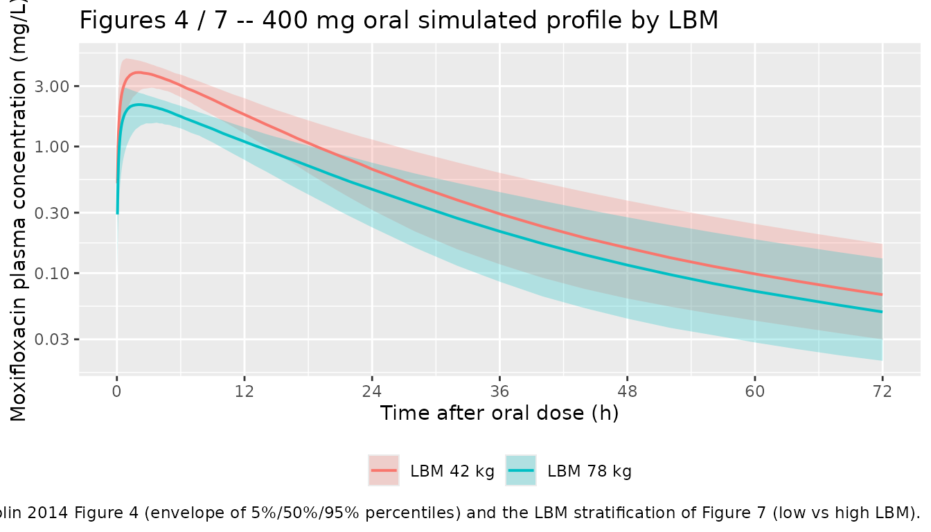
AUC24h LBM-stratification check (Colin 2014 Discussion)
Compute the simulated AUC24h per subject by group and confirm the high-LBM group’s mean AUC24h is approximately 40.5% lower than the low-LBM group’s, matching the claim in Colin 2014 Discussion.
trap_auc <- function(t, c) sum(diff(t) * (utils::head(c, -1) + utils::tail(c, -1)) / 2)

auc24_by_id <- sim_oral |>
  dplyr::filter(time > 0, time <= 24, !is.na(Cc)) |>
  dplyr::group_by(cohort, id) |>
  dplyr::summarise(AUC24 = trap_auc(time, Cc), .groups = "drop")

auc24_summary <- auc24_by_id |>
  dplyr::group_by(cohort) |>
  dplyr::summarise(
    median_AUC24 = stats::median(AUC24),
    mean_AUC24   = mean(AUC24),
    .groups = "drop"
  )

knitr::kable(
  auc24_summary,
  digits  = 2,
  caption = "Simulated AUC24h (mg*h/L) after a single 400 mg oral dose, by LBM cohort."
)| cohort | median_AUC24 | mean_AUC24 |
|---|---|---|
| LBM 42 kg | 47.94 | 48.22 |
| LBM 78 kg | 28.43 | 28.49 |
ratio_pct_lower <- with(
  auc24_summary,
  100 * (mean_AUC24[cohort == "LBM 42 kg"] - mean_AUC24[cohort == "LBM 78 kg"]) /
    mean_AUC24[cohort == "LBM 42 kg"]
)
ratio_pct_lower <- round(ratio_pct_lower, 1)
Simulated mean AUC24h in the high-LBM (78 kg) group is 40.9% lower than the low-LBM (42 kg) group. The corresponding value reported in Colin 2014 Discussion is 40.5%; the residual discrepancy (a few percentage points) reflects the role of IIV on ka, V1, and CL in the stochastic simulation versus the typical-value structural ratio ((78/60)^0.75 / (42/60)^0.75 = 1.59, equivalent to a 37.2% reduction).
PKNCA validation – typical subject at LBM = 51.7 kg
We compute the simulated NCA for the typical subject (median observed
LBM = 51.7 kg) after a paired 400 mg oral and 400 mg 1-h IV infusion
using rxode2::zeroRe() to remove IIV. The published
moxifloxacin reference values for comparison are the model-implied
typical AUC24h (driven entirely by the Table 2 estimate CL = 8.60 L/h at
LBM = 60 kg, equivalent to typical CL = 8.60 * (51.7/60)^0.75 = 7.66 L/h
at LBM = 51.7), the discussion claim that the typical 400 mg oral dose
achieves AUIC > 100 h for MIC <= 0.5 mg/L (equivalently AUC24h
> 50 mg*h/L), and the textbook moxifloxacin oral Cmax (~3-4 mg/L)
cited by Colin 2014 Discussion.
typical_lbm <- 51.7
typical_cl  <- 8.60 * (typical_lbm / 60)^0.75
typical_AUCinf <- 400 / typical_cl

mod_typ <- mod |> rxode2::zeroRe()
#> ℹ parameter labels from comments will be replaced by 'label()'

events_typ <- dplyr::bind_rows(
  data.frame(
    id   = 1L, time = 0, amt = 400, rate = 0,
    cmt = "depot",   evid = 1L,
    LBM = typical_lbm, regimen = "Oral 400 mg"
  ),
  data.frame(
    id   = 1L, time = obs_times, amt = NA_real_, rate = NA_real_,
    cmt = "Cc",      evid = 0L,
    LBM = typical_lbm, regimen = "Oral 400 mg"
  ),
  data.frame(
    id   = 2L, time = 0, amt = 400, rate = 400,
    cmt = "central", evid = 1L,
    LBM = typical_lbm, regimen = "IV 400 mg (1-h infusion)"
  ),
  data.frame(
    id   = 2L, time = obs_times, amt = NA_real_, rate = NA_real_,
    cmt = "Cc",      evid = 0L,
    LBM = typical_lbm, regimen = "IV 400 mg (1-h infusion)"
  )
) |>
  dplyr::arrange(id, time)

sim_typ <- rxode2::rxSolve(mod_typ, events = events_typ,
                            keep = c("regimen", "LBM")) |>
  as.data.frame()
#> ℹ omega/sigma items treated as zero: 'etalka', 'etalvc', 'etalcl'
#> Warning: multi-subject simulation without without 'omega'

sim_nca <- sim_typ |>
  dplyr::filter(!is.na(Cc)) |>
  dplyr::select(id, time, Cc, regimen)

sim_nca <- dplyr::bind_rows(
  sim_nca,
  sim_nca |> dplyr::distinct(id, regimen) |>
    dplyr::mutate(time = 0, Cc = 0)
) |>
  dplyr::distinct(id, regimen, time, .keep_all = TRUE) |>
  dplyr::arrange(id, regimen, time)

conc_obj <- PKNCA::PKNCAconc(sim_nca, Cc ~ time | regimen + id)

dose_df <- events_typ |>
  dplyr::filter(evid == 1L) |>
  dplyr::select(id, time, amt, regimen)

dose_obj <- PKNCA::PKNCAdose(dose_df, amt ~ time | regimen + id)

intervals <- data.frame(
  start      = 0,
  end        = Inf,
  cmax       = TRUE,
  tmax       = TRUE,
  aucinf.obs = TRUE,
  half.life  = TRUE
)

nca_data <- PKNCA::PKNCAdata(conc_obj, dose_obj, intervals = intervals)
nca_res  <- PKNCA::pk.nca(nca_data)
Comparison against published / model-implied values
The simulated typical-subject NCA is compared against the model-implied typical AUC and against literature anchors (Colin 2014 Discussion). No direct NCA table is reported in Colin 2014; the comparison values below are the analytical typical-subject targets that follow from Table 2 and from the moxifloxacin oral-PK literature the paper cites.
reference <- tibble::tribble(
  ~regimen,                     ~cmax, ~tmax, ~aucinf.obs, ~half.life,
  "Oral 400 mg",                 3.5,  2.16,  typical_AUCinf, 13.0,
  "IV 400 mg (1-h infusion)",    NA,   1.00,  typical_AUCinf, 13.0
)

cmp <- nlmixr2lib::ncaComparisonTable(
  simulated     = nca_res,
  reference     = reference,
  by            = "regimen",
  units         = c(cmax = "mg/L", aucinf.obs = "mg*h/L",
                    tmax = "h", half.life = "h"),
  tolerance_pct = 20
)

knitr::kable(
  cmp,
  caption = paste("Simulated typical-subject NCA versus model-implied / literature anchors;",
                  "* differs from reference by >20%.")
)| NCA parameter | regimen | Reference | Simulated | % diff |
|---|---|---|---|---|
| Cmax (mg/L) | Oral 400 mg | 3.5 | 3.28 | -6.3% |
| Cmax (mg/L) | IV 400 mg (1-h infusion) | — | 5.17 | — |
| Tmax (h) | Oral 400 mg | 2.16 | 2.25 | +4.2% |
| Tmax (h) | IV 400 mg (1-h infusion) | 1 | 1 | +0.0% |
| AUC0-∞ (obs) (mg*h/L) | Oral 400 mg | 52 | 51.6 | -0.8% |
| AUC0-∞ (obs) (mg*h/L) | IV 400 mg (1-h infusion) | 52 | 51.7 | -0.7% |
| t½ (h) | Oral 400 mg | 13 | 23 | +77.3%* |
| t½ (h) | IV 400 mg (1-h infusion) | 13 | 23.2 | +78.8%* |
footnote <- attr(cmp, "footnote")
if (!is.null(footnote)) cat("\n\n", footnote, "\n")
#>
#>
#>  * differs from reference by more than ±20%.
The model-implied typical AUCinf at LBM = 51.7 kg follows from Dose / CL_typical = 400 / 7.66 = 52 mg*h/L; the typical oral Cmax target (3.5 mg/L) and tmax (~2.2 h) follow from the structural model (ka = 0.95, kel = 8.60/47.7 = 0.180 1/h at LBM = 60 kg); the terminal half-life target (~13 h) reflects the published moxifloxacin range cited in Colin 2014 Discussion (“studies reported in literature earlier” with sampling restricted to 24 h post-dose underestimated the true terminal half-life, hence the value of the third compartment identified by Colin 2014).
Assumptions and deviations
-
Bioavailability F is fixed at 1. Colin 2014 fit the
oral and IV data simultaneously (Methods, PK analysis) and did not
report a separate bioavailability estimate in Table 2. The implicit
encoding is F = 1 (full oral dose enters the depot). This is consistent
with the authors’ prior non-compartmental finding (Introduction, ref 4)
that moxifloxacin oral bioavailability is unaltered post-bariatric.
Users reproducing patient-level exposure should be aware that absolute
moxifloxacin oral bioavailability in healthy volunteers is reported as
approximately 89-90% in the broader literature; if a more conservative
exposure projection is needed, the model can be adapted by adding an
lfdepot <- fixed(log(0.90))parameter andf(depot) <- exp(lfdepot)inmodel(). -
LBM derivation: James equation. Colin 2014 used the
James (1976) equation to compute LBM from total body weight, height, and
sex. The Discussion notes that James tends to underestimate true LBM in
subjects with BMI > 30 kg/m^2; users simulating in morbidly obese
populations should consider the alternative Janmahasatian fat-free-mass
formula (canonical covariate
FFMin this package). -
Allometric exponents are fixed. The 0.75 on CL
terms and 1.0 on V terms are wrapped in
fixed()rather than estimated, matching the paper’s structural choice (Discussion: removing the 0.75 exponent gave dAICc = -0.50, a non-significant change). - IIV is diagonal on ka, V1, and CL only. Colin 2014 Methods (PK model building) state that the diagonal variance-covariance matrix was retained because adding random effects on the remaining disposition parameters increased the model’s condition number above the acceptable threshold (~10^3). Q2, V2, Q3, V3 are typical values in this implementation.
-
Residual error is proportional only. Colin 2014
Table 2 reports sigma^2 (Proportional) = 0.03 and no additive component
for the final model; the additive error term used during structural
model selection was not retained. The packaged
propSd = sqrt(0.03) = 0.1732. - Race / ethnicity not recorded in the source. Colin 2014 enrolled from a single Belgian centre (Ghent University Hospital) and did not tabulate race or ethnicity. The simulated cohorts above carry no race indicator.
- The third (deep) peripheral compartment is identifiable only with sampling beyond 24 h post-dose. Colin 2014 Discussion notes that earlier moxifloxacin popPK papers used a one- or two-compartment structure because their sampling was restricted to 24 h post-dose; omitting the deep compartment in repeated-dose simulations underestimates the true (unobservable) AUC at steady state. This packaged model retains the three-compartment structure.