Evolocumab (Gibbs 2017)
Source:vignettes/articles/Gibbs_2017_evolocumab.Rmd
Gibbs_2017_evolocumab.RmdModel and source
- Citation: Gibbs JP, Doshi S, Kuchimanchi M, Grover A, Emery MG, Dodds MG, Gibbs MA, Somaratne R, Wasserman SM, Blom D. Impact of target-mediated elimination on the dose and regimen of evolocumab, a human monoclonal antibody against proprotein convertase subtilisin/kexin type 9 (PCSK9). J Clin Pharmacol. 2017;57(5):616-626. doi:10.1002/jcph.840
- Description: Target-mediated drug disposition (quasi-steady-state approximation) PK/PD model for evolocumab, an anti-PCSK9 monoclonal antibody, in healthy subjects and statin-treated patients with hypercholesterolemia (Gibbs 2017): one-compartment evolocumab disposition with first-order SC absorption, linear clearance plus PCSK9-complex-mediated (target) elimination, coupled to a PCSK9 turnover pool and to a type-4 indirect-response model in which unbound PCSK9 inhibits LDL-cholesterol elimination.
- Article: https://doi.org/10.1002/jcph.840
Evolocumab is a fully human IgG2 monoclonal antibody against proprotein convertase subtilisin/kexin type 9 (PCSK9). PCSK9 promotes degradation of the low-density lipoprotein receptor, so removing unbound PCSK9 increases LDL receptor recycling and accelerates clearance of LDL-cholesterol (LDL-C). Because PCSK9 is an abundant, high-turnover soluble target, binding to it is also a route of elimination for evolocumab itself, which is what makes the drug’s pharmacokinetics nonlinear.
Gibbs 2017 links three layers in one simultaneously-fitted model:
- a one-compartment evolocumab PK model with first-order subcutaneous (SC) absorption and linear plus target-mediated elimination, using the quasi-steady-state (QSS) approximation of the full TMDD model;
- a PCSK9 turnover pool whose degradation is accelerated by binding to evolocumab and elimination of the complex; and
- a type-4 indirect-response model for LDL-C in which unbound PCSK9 inhibits LDL-C elimination.
The paper’s purpose is a dosing question that the coupling makes counter-intuitive: doubling the dose does not buy a doubled dosing interval. Both the target-mediated PK nonlinearity and the saturable PCSK9 -> LDL-C relationship compress the benefit of a larger dose, so an approximately 3-fold dose increase (140 mg Q2W -> 420 mg QM) is needed to hold the same time-averaged LDL-C reduction over a monthly interval.
Population
The model was fitted to pooled data from two phase 1 studies in 101 individuals contributing 4910 observations of unbound evolocumab, unbound PCSK9, and LDL-C:
- Study 20080397 (phase 1a) – 44 healthy subjects, single ascending SC doses of 7, 21, 70, 210, or 420 mg.
- Study 20080398 (phase 1b) – 57 patients with hypercholesterolemia on stable low- to moderate-intensity statin therapy, multiple ascending SC doses of 14 mg QW x 6, 35 mg QW x 6, 140 mg Q2W x 3, 280 mg Q2W x 3, or 420 mg QM x 2. Two further cohorts received high-intensity statin therapy or carried a heterozygous familial hypercholesterolemia diagnosis and were dosed 140 mg Q2W x 3.
Across both studies 73 participants received evolocumab and 28 received placebo. Most were male (73.3%) and white (83.2%), with a mean age of 45.5 years and a mean body weight of 81.4 kg. Baseline PCSK9 was 1.58-fold higher in the phase 1b study than in the phase 1a study, because statins upregulate PCSK9 – the single covariate the final model retains.
Estimation used NONMEM 7.2 (SAEM followed by importance sampling), with the M3 method for below-quantification-limit unbound evolocumab and unbound PCSK9 observations.
The same information is available programmatically via the model’s
population metadata:
str(readModelDb("Gibbs_2017_evolocumab")()$population)
#> List of 15
#>  $ species       : chr "human"
#>  $ n_subjects    : int 101
#>  $ n_observations: int 4910
#>  $ n_studies     : int 2
#>  $ n_healthy     : int 44
#>  $ n_patients    : int 57
#>  $ age_mean      : chr "45.5 years"
#>  $ weight_mean   : chr "81.4 kg"
#>  $ sex_female_pct: num 26.7
#>  $ race_ethnicity: chr "83.2% white (pooled across both studies; the paper reports only the pooled white percentage)"
#>  $ disease_state : chr "Pooled: healthy subjects (phase 1a study 20080397, single ascending SC dose) and patients with hypercholesterol"| __truncated__
#>  $ dose_range    : chr "Phase 1a: single SC 7, 21, 70, 210, or 420 mg. Phase 1b: SC 14 mg QW x 6, 35 mg QW x 6, 140 mg Q2W x 3, 280 mg "| __truncated__
#>  $ pcsk9_baseline: chr "5.27 nM (379 ng/mL) typical in statin-treated patients; 3.36 nM (242 ng/mL) typical in healthy subjects. Baseli"| __truncated__
#>  $ ldlc_baseline : chr "116 mg/dL typical (BASE_LDL-C, Table 3)"
#>  $ notes         : chr "A total of 73 participants received evolocumab and 28 received placebo across the two studies; the model datase"| __truncated__
Source trace
The per-parameter origin is recorded as an in-file comment next to
each ini() entry in
inst/modeldb/specificDrugs/Gibbs_2017_evolocumab.R. The
table below collects them in one place for review.
| Equation / parameter | Value | Source location |
|---|---|---|
d/dt(depot) |
n/a | Equation 1 |
d/dt(central) (total drug amount, TDA) |
n/a | Equation 2 |
d/dt(total_target) (total ligand conc., TLC) |
n/a | Equation 3 |
tdc <- central / vc |
n/a | Equation 4 |
fdc (free drug conc., QSS quadratic root) |
n/a | Equation 5 |
flc <- tlc - (tdc - fdc) |
n/a | Equation 6 |
d/dt(ldl) |
n/a | Equation 7 |
ksyn <- kdeg * rbase_target |
n/a | Methods: “related to the baseline PCSK9 (BASE_PCSK9) level as ksyn/kdeg” |
lka |
0.245 1/day | Table 2 |
lcl |
0.256 L/day | Table 2 |
lvc |
2.66 L | Table 2 |
lfdepot |
0.72 (fixed) | Methods: “Bioavailability (F) was fixed to 72% (Amgen internal data)” |
lkdeg |
2.12 1/day | Table 2 |
lrbase_target |
5.27 nM | Table 2; Results (“5.27 nM (or 379 ng/mL)”) |
lkss |
0.253 nM | Table 2 |
lkint |
0.0529 1/day | Table 2 |
e_dis_healthy_rbase_target |
0.637 | Table 2 (theta 1); Results (“3.36 nM (or 242 ng/mL) in healthy subjects”) |
lkout |
0.305 1/day | Table 3 |
lrbase_ldl |
116 mg/dL | Table 3 |
limax |
1.00 (fixed) | Table 3; Results (“near the boundary of 1.00, so its value was fixed”) |
lic50 |
1.46 nM | Table 3; Abstract |
etalka + etalvc + etalcl block |
0.807 / 0.158 / 0.924; cov 0.253 / -0.671 / -0.183 | Table 2 random-effects and Covariance rows |
etalrbase_target |
0.0348 | Table 2 |
etalkss |
1.17 | Table 2 |
etalrbase_ldl |
0.0465 | Table 3 |
etalic50 |
0.481 | Table 3 |
propSd (unbound evolocumab) |
sqrt(0.0576) = 0.240 | Table 2 sigma^2 (evolocumab) |
propSd_freePcsk9 |
sqrt(0.0942) = 0.3069 | Table 2 sigma^2 (PCSK9) |
propSd_ldl |
sqrt(0.0130) = 0.1140 | Table 3 sigma^2 (proportional) |
addSd_ldl |
sqrt(60.1) = 7.7524 mg/dL | Table 3 sigma^2 (additive), footnote b |
MW_EVO = 141800 g/mol |
– | Not in the paper – see Assumptions and deviations |
Reading the random-effects columns
Both tables print the random-effects column as
Estimate (~CV%), and the footnote defines “CV%, coefficient
of variation calculated as sqrt(var) x 100”. The estimates are therefore
variances, carried into ini() unchanged.
Each printed CV% reproduces from the estimate, which confirms the
reading rather than assuming it:
omegas <- c(ka = 0.807, V = 0.158, CL = 0.924, BASE_PCSK9 = 0.0348,
            kss = 1.17, BASE_LDLC = 0.0465, IC50 = 0.481)
published_cv <- c(90, 40, 96, 19, 108, 22, 69)
round(sqrt(omegas) * 100)
#>         ka          V         CL BASE_PCSK9        kss  BASE_LDLC       IC50
#>         90         40         96         19        108         22         69
stopifnot(abs(round(sqrt(omegas) * 100) - published_cv) <= 1)
The parenthesised percentages on the three Covariance
rows are correlations, and they too reproduce from the covariances –
confirming the ka/V/CL block is a covariance (not a correlation) matrix,
and that it is positive definite:
blk <- matrix(c( 0.807,  0.253, -0.671,
                 0.253,  0.158, -0.183,
                -0.671, -0.183,  0.924), 3, 3,
              dimnames = list(c("ka", "V", "CL"), c("ka", "V", "CL")))
round(stats::cov2cor(blk) * 100)      # published: 70, -78, -48
#>     ka   V  CL
#> ka 100  71 -78
#> V   71 100 -48
#> CL -78 -48 100
stopifnot(
  abs(round(stats::cov2cor(blk)[1, 2] * 100) -  70) <= 1,
  abs(round(stats::cov2cor(blk)[1, 3] * 100) - -78) <= 1,
  abs(round(stats::cov2cor(blk)[2, 3] * 100) - -48) <= 1,
  # Positive definite, so rxode2's Cholesky sampler can draw from it as-is
  # (no off-diagonal nudge needed).
  all(eigen(blk, symmetric = TRUE, only.values = TRUE)$values > 0)
)
Model structure
mod <- readModelDb("Gibbs_2017_evolocumab")
mod
#> function() {
#>   description <- "Target-mediated drug disposition (quasi-steady-state approximation) PK/PD model for evolocumab, an anti-PCSK9 monoclonal antibody, in healthy subjects and statin-treated patients with hypercholesterolemia (Gibbs 2017): one-compartment evolocumab disposition with first-order SC absorption, linear clearance plus PCSK9-complex-mediated (target) elimination, coupled to a PCSK9 turnover pool and to a type-4 indirect-response model in which unbound PCSK9 inhibits LDL-cholesterol elimination."
#>   reference <- "Gibbs JP, Doshi S, Kuchimanchi M, Grover A, Emery MG, Dodds MG, Gibbs MA, Somaratne R, Wasserman SM, Blom D. Impact of target-mediated elimination on the dose and regimen of evolocumab, a human monoclonal antibody against proprotein convertase subtilisin/kexin type 9 (PCSK9). J Clin Pharmacol. 2017;57(5):616-626. doi:10.1002/jcph.840"
#>   vignette <- "Gibbs_2017_evolocumab"
#>
#>   # Time in days; doses entered in mg and converted to nmol on the dose record
#>   # (see f(depot) in model()); all drug and target concentrations are molar (nM),
#>   # matching the paper's equations 1-7 and Tables 2-3. LDL-C is in mg/dL.
#>   units <- list(time = "day", dosing = "mg", concentration = "nM")
#>
#>   # Issue #482: what each ODE state holds, in what amount units, in what
#>   # biological matrix. verified = TRUE: each entry was checked against Gibbs
#>   # 2017 equations 1-4 and 7 and the Figure 1 schematic.
#>   #
#>   # NOTE the mixed amount/concentration bases, which are the paper's own:
#>   # equations 1-2 carry evolocumab as an AMOUNT (Adepot, TDA) while equations 3
#>   # and 7 carry PCSK9 and LDL-C as CONCENTRATIONS (TLC, LDL). TDA is converted
#>   # to the concentration TDC by TDA/V (equation 4).
#>   compartmentData <- list(
#>     depot = list(analyte = "evolocumab", units = "nmol", specimen = "administration site", verified = TRUE),
#>     central = list(
#>       analyte = "total (unbound + PCSK9-bound) evolocumab",
#>       units = "nmol",
#>       specimen = "serum",
#>       verified = TRUE
#>     ),
#>     total_target = list(
#>       analyte = "total (unbound + evolocumab-bound) PCSK9",
#>       units = "nM",
#>       specimen = "serum",
#>       verified = TRUE
#>     ),
#>     ldl = list(analyte = "low-density lipoprotein cholesterol", units = "mg/dL", specimen = "serum", verified = TRUE)
#>   )
#>
#>   covariateData <- list(
#>     DIS_HEALTHY = list(
#>       description = "Healthy-participant cohort indicator, 1 = healthy subject (phase 1a study 20080397), 0 = hypercholesterolemic patient on stable statin therapy (phase 1b study 20080398)",
#>       units = "(binary)",
#>       type = "binary",
#>       reference_category = "0 (statin-treated hypercholesterolemic patient; the population in which BASE_PCSK9 = 5.27 nM was estimated)",
#>       notes = "The only covariate retained in the Gibbs 2017 final model. Multiplicative effect on the baseline PCSK9 turnover set point: BASE_PCSK9 * theta1^DIS_HEALTHY with theta1 = 0.637 (Table 2). The paper reports the two resulting typical values explicitly in the Results, which over-determines the coding and fixes the direction: 5.27 nM (379 ng/mL) in statin-treated patients and 5.27 * 0.637 = 3.36 nM (242 ng/mL) in healthy subjects. Because BASE_PCSK9 also sets ksyn (= kdeg * BASE_PCSK9) and the LDL-C baseline balance (kin), this single covariate propagates into both the target-mediated clearance of evolocumab and the achievable LDL-C reduction. Time-fixed per subject.",
#>       source_name = "theta 1 (Gibbs 2017 Table 2 footnote: 'fold change in baseline PCSK9 for healthy subjects vs statin-treated patients')"
#>     )
#>   )
#>
#>   population <- list(
#>     species = "human",
#>     n_subjects = 101L,
#>     n_observations = 4910L,
#>     n_studies = 2L,
#>     n_healthy = 44L,
#>     n_patients = 57L,
#>     age_mean = "45.5 years",
#>     weight_mean = "81.4 kg",
#>     sex_female_pct = 26.7,
#>     race_ethnicity = "83.2% white (pooled across both studies; the paper reports only the pooled white percentage)",
#>     disease_state = "Pooled: healthy subjects (phase 1a study 20080397, single ascending SC dose) and patients with hypercholesterolemia on stable low- to moderate-intensity statin therapy (phase 1b study 20080398, multiple ascending SC dose). Two additional phase 1b cohorts received high-intensity statin therapy or carried a heterozygous familial hypercholesterolemia diagnosis and were dosed 140 mg Q2W x 3.",
#>     dose_range = "Phase 1a: single SC 7, 21, 70, 210, or 420 mg. Phase 1b: SC 14 mg QW x 6, 35 mg QW x 6, 140 mg Q2W x 3, 280 mg Q2W x 3, or 420 mg QM x 2.",
#>     pcsk9_baseline = "5.27 nM (379 ng/mL) typical in statin-treated patients; 3.36 nM (242 ng/mL) typical in healthy subjects. Baseline PCSK9 was 1.58-fold higher in the phase 1b study than the phase 1a study.",
#>     ldlc_baseline = "116 mg/dL typical (BASE_LDL-C, Table 3)",
#>     notes = "A total of 73 participants received evolocumab and 28 received placebo across the two studies; the model dataset comprised the 101 individuals with evaluable PK/PD data. Baseline demographics are given in the paper's Table S1 (Supporting Information), which was not available when this model was built; the demographic values recorded here are the pooled summaries stated in the Results narrative. Estimation used NONMEM 7.2 with SAEM followed by importance sampling, and the M3 method for below-limit-of-quantification unbound evolocumab and unbound PCSK9 observations."
#>   )
#>
#>   ini({
#>     # ================= Evolocumab PK (Gibbs 2017 Table 2) =================
#>     # One-compartment disposition, first-order SC absorption. Reference
#>     # subject for BASE_PCSK9 is the statin-treated patient (DIS_HEALTHY = 0).
#>     lka     <- log(0.245);        label("First-order SC absorption rate constant ka (1/day)")                  # Table 2: ka = 0.245 1/day (RSE 12%)
#>     lcl     <- log(0.256);        label("Linear (non-target-mediated) clearance CL (L/day)")                    # Table 2: CL = 0.256 L/day (RSE 17%)
#>     lvc     <- log(2.66);         label("Central volume of distribution V (L)")                                 # Table 2: V = 2.66 L (RSE 5.9%)
#>     lfdepot <- fixed(log(0.72));  label("Subcutaneous bioavailability F (fraction)")                            # Methods: "Bioavailability (F) was fixed to 72% (Amgen internal data)"
#>
#>     # ================= PCSK9 target turnover and binding (Table 2) =================
#>     lkdeg         <- log(2.12);   label("First-order PCSK9 degradation rate constant kdeg (1/day)")             # Table 2: kdeg = 2.12 1/day (RSE 7.3%); Discussion: "elimination half-life of approximately 8 hours"
#>     lrbase_target <- log(5.27);   label("Baseline total PCSK9 concentration BASE_PCSK9 in statin-treated patients (nM)") # Table 2: BASE_PCSK9 = 5.27 nM (RSE 2.7%); Results: "5.27 nM (or 379 ng/mL) in hypercholesterolemic patients stably treated with statins"
#>     lkss          <- log(0.253);  label("Quasi-steady-state constant kss = (kint + koff)/kon (nM)")             # Table 2: kss = 0.253 nM (RSE 23%)
#>     lkint         <- log(0.0529); label("Evolocumab-PCSK9 complex elimination (internalisation) rate constant kint (1/day)") # Table 2: kint = 0.0529 1/day (RSE 3.5%)
#>
#>     # ---- Covariate effect (Table 2, theta 1) ----
#>     e_dis_healthy_rbase_target <- 0.637; label("Fold change in baseline PCSK9 for healthy subjects vs statin-treated patients (unitless)") # Table 2: theta1 = 0.637 (RSE 4.1%); Results: 5.27 * 0.637 = 3.36 nM (242 ng/mL) in healthy subjects
#>
#>     # ================= LDL-C indirect response (Gibbs 2017 Table 3) =================
#>     lkout      <- log(0.305);      label("Maximal first-order LDL-C elimination rate constant kout, i.e. in the absence of PCSK9 (1/day)") # Table 3: kout = 0.305 1/day (RSE 4.0%); Discussion: "half-life of approximately 2.3 days ... in the absence of PCSK9"
#>     lrbase_ldl <- log(116);        label("Baseline LDL-C concentration BASE_LDL-C (mg/dL)")                      # Table 3: BASE_LDL-C = 116 mg/dL (RSE 2.9%)
#>     limax      <- fixed(log(1.00)); label("Maximal proportional inhibition of kout by PCSK9, Imax (unitless)")   # Table 3: Imax = 1.00 (fix); Results: "Initial attempts to estimate Imax suggested that it was near the boundary of 1.00, so its value was fixed to 1.00"
#>     lic50      <- log(1.46);       label("Unbound PCSK9 concentration giving half-maximal inhibition of kout, IC50 (nM)") # Table 3: IC50 = 1.46 nM (RSE 10%); Abstract: "IC50 ... was 1.46 nM"
#>
#>     # ================= Between-subject variability =================
#>     # Gibbs 2017 Tables 2-3 report the random-effects column as VARIANCES: the
#>     # table footnote defines "CV%, coefficient of variation calculated as
#>     # sqrt(var) * 100", and every printed CV% reproduces as sqrt(estimate):
#>     #   sqrt(0.807)  = 0.898 -> 90%  (ka)
#>     #   sqrt(0.158)  = 0.397 -> 40%  (V)
#>     #   sqrt(0.924)  = 0.961 -> 96%  (CL)
#>     #   sqrt(0.0348) = 0.187 -> 19%  (BASE_PCSK9)
#>     #   sqrt(1.17)   = 1.082 -> 108% (kss)
#>     #   sqrt(0.0465) = 0.216 -> 22%  (BASE_LDL-C)
#>     #   sqrt(0.481)  = 0.694 -> 69%  (IC50)
#>     # so the estimates are carried through unchanged (no CV% -> omega^2
#>     # back-transform is needed or appropriate here).
#>     #
#>     # Full 3x3 block on ka, V, CL (Table 2 "Covariance" rows). The parenthesised
#>     # percentages on those rows are correlations, and they reproduce from the
#>     # covariances, confirming the block is a covariance (not correlation) matrix:
#>     #   0.253 / sqrt(0.807 * 0.158) =  0.709 ->  70%
#>     #  -0.671 / sqrt(0.807 * 0.924) = -0.777 -> -78%
#>     #  -0.183 / sqrt(0.158 * 0.924) = -0.479 -> -48%
#>     # Lower-triangle order below is var(ka); cov(ka,V), var(V); cov(ka,CL), cov(V,CL), var(CL).
#>     etalka + etalvc + etalcl ~ c(0.807,
#>                                  0.253, 0.158,
#>                                 -0.671, -0.183, 0.924)   # Table 2: variances 0.807 / 0.158 / 0.924 and covariances 0.253 / -0.671 / -0.183
#>     etalrbase_target ~ 0.0348   # Table 2: BASE_PCSK9 intersubject variance 0.0348 (~19% CV)
#>     etalkss          ~ 1.17     # Table 2: kss intersubject variance 1.17 (~108% CV)
#>     etalrbase_ldl    ~ 0.0465   # Table 3: BASE_LDL-C intersubject variance 0.0465 (~22% CV)
#>     etalic50         ~ 0.481    # Table 3: IC50 intersubject variance 0.481 (~69% CV)
#>     # kdeg, kint, theta1, kout and Imax carry no between-subject variability:
#>     # Tables 2-3 report 0.00 with footnote a, "Intersubject random variance was
#>     # fixed at 0", and Methods states "BSV for kdeg and kint were fixed at 0%".
#>
#>     # ================= Residual unexplained variability =================
#>     # Tables 2-3 report sigma^2 (variances); nlmixr2 expects standard deviations,
#>     # so each value below is sqrt(sigma^2), and each reproduces the paper's own
#>     # parenthesised summary.
#>     propSd            <- 0.240;  label("Proportional residual error on unbound evolocumab (fraction)")  # Table 2: sigma^2 (evolocumab) = 0.0576 -> sqrt = 0.240; Results: "residual variabilities for unbound evolocumab ... were 24%"
#>     propSd_freePcsk9  <- 0.3069; label("Proportional residual error on unbound PCSK9 (fraction)")        # Table 2: sigma^2 (PCSK9) = 0.0942 -> sqrt = 0.30692; Results: "... and unbound PCSK9 were 24% and 31%"
#>     propSd_ldl        <- 0.1140; label("Proportional residual error on LDL-C (fraction)")                # Table 3: sigma^2 (proportional error) = 0.0130 -> sqrt = 0.11402; Results: "proportional and additive residual variability of 11% and 7.8 mg/dL"
#>     addSd_ldl         <- 7.7524; label("Additive residual error on LDL-C (mg/dL)")                       # Table 3: sigma^2 (additive error) = 60.1 -> sqrt = 7.7524, and the table's own parenthesised 7.8 is flagged by footnote b as "the standard deviation ... calculated as sqrt(var)"
#>   })
#>
#>   model({
#>     # ---- Physical constants ----------------------------------------------
#>     # Evolocumab molecular weight. NOT reported in Gibbs 2017: the paper works
#>     # entirely in molar units and never prints a mg <-> nmol bridge, but doses
#>     # are administered in mg, so one is required. 141,800 g/mol is the value in
#>     # the FDA-approved Repatha (evolocumab) prescribing information, and is the
#>     # same constant already used by the sibling registry model
#>     # inst/modeldb/specificDrugs/Kuchimanchi_2018_evolocumab.R (MW_EVO).
#>     # Non-paper provenance; see the vignette's Assumptions and deviations
#>     # section, which also shows that the paper's reported simulation endpoints
#>     # move by < 1 percentage point when this constant is varied to 150,000.
#>     MW_EVO      <- 141800        # g/mol
#>     nmol_per_mg <- 1e6 / MW_EVO  # 7.052 nmol per mg
#>
#>     # ---- Individual PK parameters (Table 2) -------------------------------
#>     ka     <- exp(lka + etalka)
#>     cl     <- exp(lcl + etalcl)
#>     vc     <- exp(lvc + etalvc)
#>     fdepot <- exp(lfdepot)
#>     kdeg   <- exp(lkdeg)
#>     kint   <- exp(lkint)
#>     kss    <- exp(lkss + etalkss)
#>
#>     # Baseline PCSK9 set point. theta1 multiplies BASE_PCSK9 for healthy
#>     # subjects; the statin-treated patient (DIS_HEALTHY = 0) is the reference.
#>     rbase_target <- exp(lrbase_target + etalrbase_target) *
#>                     e_dis_healthy_rbase_target^DIS_HEALTHY
#>
#>     # Zero-order PCSK9 production. Methods: ksyn and kdeg are "related to the
#>     # baseline PCSK9 (BASE_PCSK9) level as ksyn/kdeg", i.e. ksyn = kdeg * BASE.
#>     ksyn <- kdeg * rbase_target
#>
#>     # ---- Individual PD parameters (Table 3) -------------------------------
#>     kout      <- exp(lkout)
#>     imax      <- exp(limax)
#>     ic50      <- exp(lic50 + etalic50)
#>     rbase_ldl <- exp(lrbase_ldl + etalrbase_ldl)
#>
#>     # Zero-order LDL-C production, set so that the LDL-C state holds at
#>     # BASE_LDL-C in the drug-free state, where unbound PCSK9 = BASE_PCSK9:
#>     #   0 = kin - kout * (1 - Imax * BASE_PCSK9/(IC50 + BASE_PCSK9)) * BASE_LDL-C
#>     kin <- kout * (1 - imax * rbase_target / (ic50 + rbase_target)) * rbase_ldl
#>
#>     # ---- Quasi-steady-state TMDD algebra (Gibbs 2017 equations 4-6) -------
#>     # tdc: total drug concentration = TDA / V                     (equation 4)
#>     # fdc: free (unbound) drug concentration                      (equation 5)
#>     # flc: free (unbound) ligand [PCSK9] concentration            (equation 6)
#>     # Equation 5 is the positive root of the one-to-one QSS binding quadratic
#>     #   FDC^2 + FDC * (TLC - TDC + kss) - kss * TDC = 0,
#>     # so FDC = 0.5 * [(TDC - TLC - kss) + sqrt((TDC - TLC - kss)^2 + 4*kss*TDC)].
#>     # The drug-target complex concentration is TDC - FDC, hence equation 6.
#>     tdc <- central / vc
#>     tlc <- total_target
#>     qss <- tdc - tlc - kss
#>     fdc <- 0.5 * (qss + sqrt(qss * qss + 4 * kss * tdc))
#>     flc <- tlc - (tdc - fdc)
#>
#>     # ---- ODE system (Gibbs 2017 equations 1-3 and 7, Figure 1) ------------
#>     # Equation 2 is written by the authors as "- k * FDC * V - kint * TLC * FDC * V/(kss + FDC)";
#>     # k is the first-order elimination rate constant kel = CL/V, so k * FDC * V = CL * FDC.
#>     d/dt(depot)        <- -ka * depot
#>     d/dt(central)      <-  ka * depot -
#>                            cl * fdc -
#>                            kint * tlc * fdc * vc / (kss + fdc)
#>     d/dt(total_target) <-  ksyn - kdeg * tlc -
#>                            (kint - kdeg) * fdc * tlc / (kss + fdc)
#>     d/dt(ldl)          <-  kin - kout * (1 - imax * flc / (ic50 + flc)) * ldl
#>
#>     # Initial conditions: both turnover pools start at their drug-free baselines.
#>     total_target(0) <- rbase_target
#>     ldl(0)          <- rbase_ldl
#>
#>     # SC bioavailability, combined with the mg -> nmol conversion so that dose
#>     # records are entered in mg while the compartments are molar.
#>     f(depot) <- fdepot * nmol_per_mg
#>
#>     # ---- Observations and residual error ---------------------------------
#>     # The three measured analytes are unbound evolocumab, unbound PCSK9 (both
#>     # nM; the assays deliberately do not detect the drug-target complex, see
#>     # Methods "PK/PD Sampling and Assays"), and LDL-C (mg/dL).
#>     Cc         <- fdc
#>     freePcsk9  <- flc
#>
#>     Cc        ~ prop(propSd)
#>     freePcsk9 ~ prop(propSd_freePcsk9)
#>     ldl       ~ add(addSd_ldl) + prop(propSd_ldl)
#>   })
#> }
#> <environment: 0x55679cf49800>
Equation 5 is the positive root of the one-to-one QSS binding
quadratic. With RC the complex concentration, QSS binding
gives RC = FDC * FLC / kss, and mass balance gives
FLC = TLC - RC and RC = TDC - FDC; eliminating
RC and FLC yields
FDC^2 + FDC * (TLC - TDC + kss) - kss * TDC = 0whose positive root is the printed equation 5. The PDF text layer
loses the radical and the squared term of that expression, so it was
re-derived here and checked against the printed 4 kss TDC
term, which it reproduces exactly.
A useful consequence, used repeatedly below: with Imax
fixed at 1, the maximum attainable LDL-C reduction (complete PCSK9
suppression) is BASE_PCSK9 / (IC50 + BASE_PCSK9).
max_reduction <- 5.27 / (1.46 + 5.27)
round(100 * max_reduction, 1)
#> [1] 78.3
Typical-value replication
Gibbs 2017 performed its dose-regimen simulations deterministically –
“we performed simulations using the typical values of PK/PD parameters
using Berkley Madonna” – so the replications below use
rxode2::zeroRe() to match that. The stochastic cohort comes
afterwards.
mod_typ <- rxode2::zeroRe(mod)
#> ℹ parameter labels from comments will be replaced by 'label()'

# This is a three-endpoint model (Cc, freePcsk9, ldl), so every event table
# below is built as an explicit data frame with `evid`, `cmt` and `dvid`
# columns: an observation row that names no compartment cannot be mapped to an
# endpoint and rxSolve rejects it ("'dvid'->'cmt' ... on observation record").
# Observations are placed on the ODE state `central` -- never on an algebraic
# observable name such as "Cc", which would inject an extra compartment slot
# and renumber the states -- and every model variable is returned as its own
# column regardless of which endpoint `dvid` names. `useLinCmt = FALSE` is
# required for the same reason.
make_events <- function(amt, ii, addl, until, dis_healthy = 0,
                        by = 0.05, id = 1L) {
  obs <- data.frame(id = id, time = seq(0, until, by = by), amt = NA_real_,
                    evid = 0L, cmt = "central", dvid = 1L,
                    DIS_HEALTHY = dis_healthy)
  if (is.null(amt) || amt <= 0) return(obs[order(obs$time), ])
  dose <- data.frame(id = id, time = ii * seq(0, addl), amt = amt, evid = 1L,
                     cmt = "depot", dvid = NA_integer_,
                     DIS_HEALTHY = dis_healthy)
  ev <- rbind(dose, obs)
  ev[order(ev$time, -ev$evid), ]
}

# Solve one regimen for one baseline-PCSK9 state.
# DIS_HEALTHY = 0 is the statin-treated patient (BASE_PCSK9 = 5.27 nM).
solve_regimen <- function(amt, ii, addl, until, dis_healthy = 0,
                          model = mod_typ, by = 0.05) {
  rxode2::rxSolve(
    model, make_events(amt, ii, addl, until, dis_healthy, by = by),
    useLinCmt = FALSE, returnType = "data.frame"
  )
}
Baseline holds exactly with no drug
Both turnover pools are initialised at their drug-free steady states
(ksyn = kdeg * BASE_PCSK9, and kin solved from
the LDL-C balance), so an undosed solve must be flat. This is a pure
numerical identity – the two sides share the same parameters – so a
tight bound is the correct assertion here.
hold <- solve_regimen(amt = 0, ii = 0, addl = 0, until = 120)
#> ℹ omega/sigma items treated as zero: 'etalka', 'etalvc', 'etalcl', 'etalrbase_target', 'etalkss', 'etalrbase_ldl', 'etalic50'
c(max_ldl_drift   = max(abs(hold$ldl - 116)),
  max_pcsk9_drift = max(abs(hold$total_target - 5.27)))
#>   max_ldl_drift max_pcsk9_drift
#>    5.258016e-13    4.440892e-15
stopifnot(
  max(abs(hold$ldl - 116)) < 1e-6,
  max(abs(hold$total_target - 5.27)) < 1e-6,
  # Free and total PCSK9 coincide when no drug is present (equation 6 with TDC = 0).
  max(abs(hold$freePcsk9 - hold$total_target)) < 1e-9
)
The healthy-subject covariate reproduces the paper’s second baseline
The paper prints both typical baselines, which over-determines the
coding of DIS_HEALTHY and fixes its direction.
hold_hv <- solve_regimen(amt = 0, ii = 0, addl = 0, until = 10, dis_healthy = 1)
#> ℹ omega/sigma items treated as zero: 'etalka', 'etalvc', 'etalcl', 'etalrbase_target', 'etalkss', 'etalrbase_ldl', 'etalic50'
c(patient_nM = hold$total_target[1], healthy_nM = hold_hv$total_target[1])
#> patient_nM healthy_nM
#>    5.27000    3.35699
stopifnot(
  abs(hold$total_target[1]    - 5.27) < 1e-6,   # Results: 5.27 nM (379 ng/mL)
  abs(hold_hv$total_target[1] - 3.36) < 0.01    # Results: 3.36 nM (242 ng/mL)
)
The paper’s ng/mL <-> nM conversions are internally consistent and imply a PCSK9 molecular weight of about 72 kDa (379/5.27 = 71.9; 242/3.36 = 72.0), which is used below wherever PCSK9 must be expressed in ng/mL.
Figure 5 – LDL-C time course after multiple SC doses
Replicates Figure 5 of Gibbs 2017: the time course of LDL-C over 12 weeks in statin-treated patients (BASE_PCSK9 = 5.27 nM) at 140 mg SC Q2W, 280 mg SC QM, and 420 mg SC QM.
arms <- tibble::tribble(
  ~regimen,       ~amt, ~ii, ~addl,
  "140 mg Q2W",    140,  14,     5,   # doses at weeks 0, 2, 4, 6, 8, 10
  "280 mg QM",     280,  28,     2,   # doses at weeks 0, 4, 8
  "420 mg QM",     420,  28,     2
)

fig5 <- do.call(rbind, lapply(seq_len(nrow(arms)), function(i) {
  s <- solve_regimen(arms$amt[i], arms$ii[i], arms$addl[i], until = 84)
  data.frame(regimen = arms$regimen[i], time = s$time, ldl = s$ldl,
             freePcsk9 = s$freePcsk9, Cc = s$Cc)
}))
#> ℹ omega/sigma items treated as zero: 'etalka', 'etalvc', 'etalcl', 'etalrbase_target', 'etalkss', 'etalrbase_ldl', 'etalic50'
#> ℹ omega/sigma items treated as zero: 'etalka', 'etalvc', 'etalcl', 'etalrbase_target', 'etalkss', 'etalrbase_ldl', 'etalic50'
#> ℹ omega/sigma items treated as zero: 'etalka', 'etalvc', 'etalcl', 'etalrbase_target', 'etalkss', 'etalrbase_ldl', 'etalic50'

ggplot(fig5, aes(time / 7, ldl, colour = regimen)) +
  geom_line(linewidth = 0.7) +
  geom_hline(yintercept = 116, linetype = "dotted") +
  geom_hline(yintercept = 116 * (1 - max_reduction), linetype = "dashed") +
  scale_x_continuous(breaks = seq(0, 12, 2)) +
  labs(x = "Time (weeks)", y = "LDL-C (mg/dL)", colour = NULL,
       title = "Figure 5 - LDL-C after multiple SC evolocumab doses",
       caption = paste("Replicates Figure 5 of Gibbs 2017. Dotted = baseline 116 mg/dL;",
                       "dashed = complete-PCSK9-suppression floor.")) +
  theme_bw() + theme(legend.position = "top")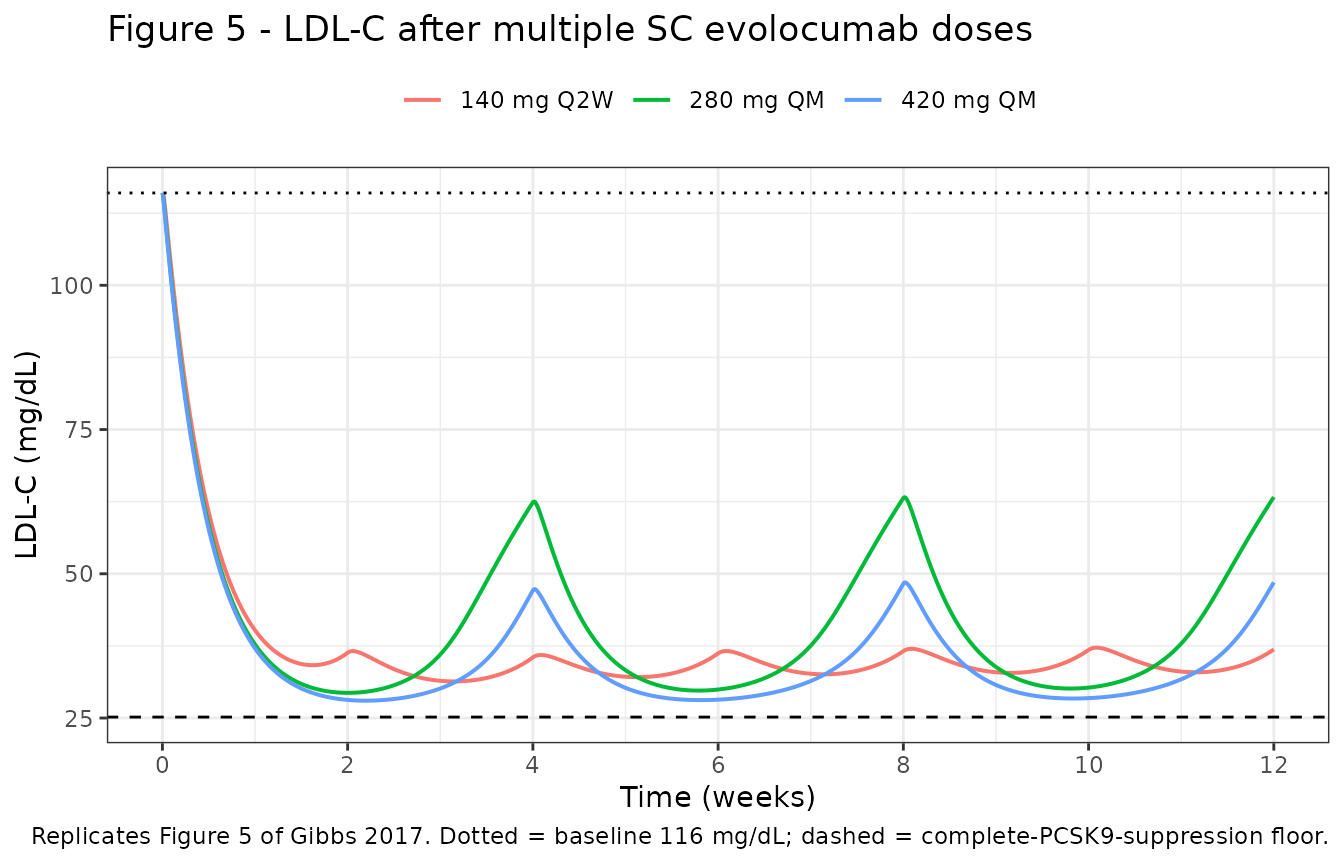
Time-averaged LDL-C reduction (the paper’s headline numbers)
Gibbs 2017 reports the time-averaged effect over the steady-state window (weeks 8 to 12) as 68.9% for 140 mg Q2W, 63.5% for 280 mg QM, and 68.9% for 420 mg QM – the quantitative basis for its “3-fold dose increase for a 2-fold interval extension” conclusion.
tavg <- fig5 |>
  filter(time >= 56, time <= 84) |>
  group_by(regimen) |>
  summarise(
    simulated_pct = mean(100 * (1 - ldl / 116)),
    trough_pct    = min(100 * (1 - ldl / 116)),
    nadir_pct     = max(100 * (1 - ldl / 116)),
    .groups = "drop"
  ) |>
  left_join(
    tibble::tibble(regimen  = c("140 mg Q2W", "280 mg QM", "420 mg QM"),
                   published_pct = c(68.9, 63.5, 68.9)),
    by = "regimen"
  ) |>
  mutate(difference_pp = simulated_pct - published_pct)

tavg |>
  mutate(across(where(is.numeric), \(x) round(x, 1))) |>
  dplyr::rename(
    "Regimen"                          = regimen,
    "Simulated time-averaged (%)"      = simulated_pct,
    "Trough (%)"                       = trough_pct,
    "Nadir (%)"                        = nadir_pct,
    "Published (%)"                    = published_pct,
    "Difference (percentage points)"   = difference_pp
  ) |>
  knitr::kable(
    caption = paste("Time-averaged LDL-C reduction over weeks 8-12 versus the values",
                    "reported in Gibbs 2017 Results.")
)| Regimen | Simulated time-averaged (%) | Trough (%) | Nadir (%) | Published (%) | Difference (percentage points) |
|---|---|---|---|---|---|
| 140 mg Q2W | 70.3 | 67.9 | 71.7 | 68.9 | 1.4 |
| 280 mg QM | 65.5 | 45.4 | 74.0 | 63.5 | 2.0 |
| 420 mg QM | 70.9 | 58.2 | 75.5 | 68.9 | 2.0 |
The reproduction is within about 2 percentage points on all three arms, and reproduces the paper’s two structural conclusions exactly: 280 mg QM is the clear loser, and 140 mg Q2W and 420 mg QM are equivalent.
These assertions are safe to keep tight because this whole section is
deterministic – zeroRe() removes every random effect, so
there is no cohort draw to vary across rxode2 builds or CI thread
counts.
stopifnot(
  # Each arm reproduces its published value. Observed differences at authoring:
  # +1.4, +2.0, +2.0 percentage points; the bound leaves headroom but a
  # mis-transcribed CL, IC50, dose or unit conversion moves these by tens of points.
  all(abs(tavg$difference_pp) < 3.5),
  # Conclusion 1: 280 mg QM is materially worse than either of the other arms.
  # Observed gaps at authoring: 4.8 and 5.4 percentage points; published: 5.4 both.
  with(tavg, simulated_pct[regimen == "140 mg Q2W"] -
             simulated_pct[regimen == "280 mg QM"]) > 3,
  with(tavg, simulated_pct[regimen == "420 mg QM"] -
             simulated_pct[regimen == "280 mg QM"]) > 3,
  # Conclusion 2: 140 mg Q2W and 420 mg QM are equivalent (published: both 68.9%).
  # Observed gap at authoring: 0.7 percentage points.
  with(tavg, abs(simulated_pct[regimen == "140 mg Q2W"] -
                 simulated_pct[regimen == "420 mg QM"])) < 2,
  # Conclusion 3: 280 mg QM fails by fluctuating over the interval, not by a
  # lower peak effect -- its nadir is comparable while its trough is far worse.
  with(tavg, trough_pct[regimen == "280 mg QM"] <
             trough_pct[regimen == "140 mg Q2W"] - 15)
)
Unbound PCSK9 suppression and its duration
The paper makes two separate observational claims about the single-dose study: that doses of 21 mg and above produced “> 80% suppression of unbound PCSK9”, and that “the duration of full suppression” rose with dose “up to a maximum of 14 days” at 420 mg. The two are different thresholds – full suppression means unbound PCSK9 driven below the assay’s lower limit of quantification (15 ng/mL), which from a 3.36 nM healthy baseline is a 93.8% reduction.
lloq_pcsk9_nM <- 15 / mw_pcsk9_kda   # 15 ng/mL assay LLOQ -> nM

single_doses <- c(7, 21, 70, 210, 420)
supp <- do.call(rbind, lapply(single_doses, function(d) {
  s <- solve_regimen(d, ii = 0, addl = 0, until = 90, dis_healthy = 1)
  base_hv <- s$total_target[1]
  blq <- s$freePcsk9 < lloq_pcsk9_nM
  data.frame(
    dose_mg         = d,
    max_suppression = 100 * (1 - min(s$freePcsk9) / base_hv),
    days_full_supp  = if (any(blq)) max(s$time[blq]) else 0
  )
}))
#> ℹ omega/sigma items treated as zero: 'etalka', 'etalvc', 'etalcl', 'etalrbase_target', 'etalkss', 'etalrbase_ldl', 'etalic50'
#> ℹ omega/sigma items treated as zero: 'etalka', 'etalvc', 'etalcl', 'etalrbase_target', 'etalkss', 'etalrbase_ldl', 'etalic50'
#> ℹ omega/sigma items treated as zero: 'etalka', 'etalvc', 'etalcl', 'etalrbase_target', 'etalkss', 'etalrbase_ldl', 'etalic50'
#> ℹ omega/sigma items treated as zero: 'etalka', 'etalvc', 'etalcl', 'etalrbase_target', 'etalkss', 'etalrbase_ldl', 'etalic50'
#> ℹ omega/sigma items treated as zero: 'etalka', 'etalvc', 'etalcl', 'etalrbase_target', 'etalkss', 'etalrbase_ldl', 'etalic50'
supp |>
  mutate(across(where(is.numeric), \(x) round(x, 1))) |>
  dplyr::rename("Single SC dose (mg)"                   = dose_mg,
                "Maximum PCSK9 suppression (%)"         = max_suppression,
                "Days of full suppression (< 15 ng/mL)" = days_full_supp) |>
  knitr::kable(caption = paste("Unbound PCSK9 suppression after a single SC dose in",
"healthy subjects (typical-value prediction)."))| Single SC dose (mg) | Maximum PCSK9 suppression (%) | Days of full suppression (< 15 ng/mL) |
|---|---|---|
| 7 | 31.1 | 0.0 |
| 21 | 76.0 | 0.0 |
| 70 | 96.5 | 5.5 |
| 210 | 99.0 | 14.7 |
| 420 | 99.5 | 20.8 |
The dose-ordering and the depth of suppression reproduce, and the 7 mg dose correctly fails to suppress – consistent with the paper’s report that unbound evolocumab was below the detection limit in every healthy subject after 7 mg. Two quantitative details do not reproduce exactly and are recorded as known deviations rather than gated: the typical-value prediction reaches 76% suppression at 21 mg where the paper reports “> 80%”, and it holds full suppression for about 21 days at 420 mg where the paper reports a maximum of 14 days. Both published numbers summarise observed data read off a discrete visit schedule (days 1, 3, 4, 5, 6, 7, 8, 11, 15, 22, 29, …), so their resolution near 14 days is roughly a week, and both are individual-level observations rather than typical-value predictions. See Assumptions and deviations.
stopifnot(
  # Deep suppression at the doses where the paper's claim is unambiguous.
  all(supp$max_suppression[supp$dose_mg >= 70] > 90),
  # The 7 mg dose does not meaningfully suppress; 21 mg clearly does.
  supp$max_suppression[supp$dose_mg == 7]  < 50,
  supp$max_suppression[supp$dose_mg == 21] > 60,
  # Both metrics rise monotonically with dose (the paper's stated trend).
  all(diff(supp$max_suppression) > 0),
  all(diff(supp$days_full_supp) >= 0),
  # Full suppression at 420 mg lasts on the order of the published 14 days
  # (deterministic, so this window is a real gate, not a formality).
  supp$days_full_supp[supp$dose_mg == 420] > 7,
  supp$days_full_supp[supp$dose_mg == 420] < 35
)
Virtual cohort and stochastic simulation
The section above is deterministic. To exercise the published between-subject variability – which is large (CV 96% on CL, 108% on kss) – the cohort below simulates the phase 1b 140 mg Q2W x 3 regimen with all random effects active.
# `set.seed()` seeds R's RNG, NOT rxode2's simulation RNG, and rxode2's streams
# are partitioned per solver thread -- so this cohort is reproducible on this
# machine and different on a machine with a different thread count. Every
# assertion below is therefore written on medians and robust quantiles, never
# on a cohort extreme.
set.seed(20170840)
rxode2::rxSetSeed(20170840)

n_per_arm <- 200L   # cohort cap is 200 per arm

make_cohort <- function(n, dis_healthy, label, id_offset = 0L) {
  do.call(rbind, lapply(seq_len(n), function(i) {
    ev <- make_events(amt = 140, ii = 14, addl = 2, until = 85,
                      dis_healthy = dis_healthy, by = 0.5,
                      id = id_offset + i)
    ev$cohort <- label
    ev
  }))
}

events <- rbind(
  make_cohort(n_per_arm, 0, "Statin-treated patients", id_offset =   0L),
  make_cohort(n_per_arm, 1, "Healthy subjects",        id_offset = 200L)
)
stopifnot(!anyDuplicated(unique(events[, c("id", "time", "evid")])))
sim <- rxode2::rxSolve(
  mod, events = events,
  keep = c("cohort", "DIS_HEALTHY"),
  useLinCmt = FALSE
) |> as.data.frame()
#> ℹ parameter labels from comments will be replaced by 'label()'

# The QSS free-drug root involves a square root; confirm the solve produced no
# NaN anywhere before any of it is summarised.
stopifnot(
  all(is.finite(sim$Cc)), all(is.finite(sim$freePcsk9)), all(is.finite(sim$ldl)),
  all(sim$Cc >= -1e-8), all(sim$freePcsk9 >= -1e-8), all(sim$ldl > 0),
  # Free ligand can never exceed total ligand (equations 5 and 6).
  all(sim$freePcsk9 <= sim$total_target + 1e-8)
)
Figure 4B – visual predictive check, 140 mg SC Q2W x 3
Replicates Figure 4B of Gibbs 2017: median and 90% prediction interval for unbound evolocumab, unbound PCSK9, and LDL-C in the statin-treated cohort.
vpc <- sim |>
  filter(cohort == "Statin-treated patients") |>
  select(time, Cc, freePcsk9, ldl) |>
  pivot_longer(-time, names_to = "analyte", values_to = "value") |>
  mutate(analyte = factor(
    analyte,
    levels = c("Cc", "freePcsk9", "ldl"),
    labels = c("Unbound evolocumab (nM)", "Unbound PCSK9 (nM)", "LDL-C (mg/dL)")
  )) |>
  group_by(analyte, time) |>
  summarise(Q05 = quantile(value, 0.05), Q50 = median(value),
            Q95 = quantile(value, 0.95), .groups = "drop")

ggplot(vpc, aes(time, Q50)) +
  geom_ribbon(aes(ymin = Q05, ymax = Q95), alpha = 0.25, fill = "steelblue") +
  geom_line(linewidth = 0.7) +
  facet_wrap(~analyte, scales = "free_y") +
  labs(x = "Time (days)", y = NULL,
       title = "Figure 4B - VPC, 140 mg SC evolocumab Q2W x 3",
       caption = "Replicates Figure 4B of Gibbs 2017 (median and 90% prediction interval).") +
  theme_bw()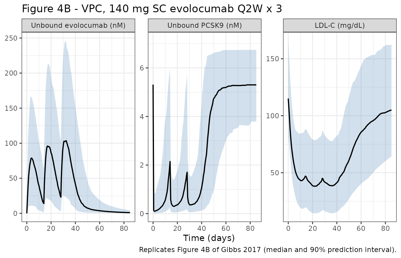
# Robust, median-based checks only -- these must hold for ANY cohort the model
# can draw, so nothing here depends on which subjects landed in the tails.
ldl_med <- vpc |>
  filter(analyte == "LDL-C (mg/dL)", time >= 28, time <= 42) |>
  summarise(reduction = mean(100 * (1 - Q50 / 116))) |>
  pull(reduction)

stopifnot(
  # The median subject's LDL-C reduction after 3 doses sits in the same region
  # as the deterministic prediction, well short of the structural ceiling.
  ldl_med > 40, ldl_med < 100 * max_reduction + 1,
  # PCSK9 is deeply suppressed at the median right after a dose ...
  min(vpc$Q50[vpc$analyte == "Unbound PCSK9 (nM)"]) < 1,
  # ... and the median recovers toward, but does not overshoot, baseline by the
  # end of follow-up. Paper: "returned toward the baseline without evidence of
  # rebound above the initial baseline values."
  max(vpc$Q50[vpc$analyte == "Unbound PCSK9 (nM)"]) < 5.27 * 1.05
)
Statin intensity as a target-mediated-elimination falsifier
Gibbs 2017 Table 1 reports a within-study contrast that is a strong, schedule-independent check on the whole TMDD layer: among patients given 140 mg Q2W, those on high-intensity statins had 26% higher baseline PCSK9 (487 vs 385 ng/mL) and, consequently, 20% lower unbound evolocumab Cmax and AUClast (ratios 0.80 and 0.80). A model with a mis-specified target sink would not reproduce that coupling.
The two strata differ only in baseline PCSK9, so they are simulated
by setting lrbase_target to each stratum’s observed value
rather than by a covariate.
strata <- tibble::tibble(
  treatment      = c("Low-moderate intensity statin", "High intensity statin"),
  pcsk9_ng_ml    = c(385, 487),
  base_nM        = c(385, 487) / mw_pcsk9_kda   # paper's own ng/mL <-> nM bridge
)

mw_evo <- 141800   # g/mol; see Assumptions and deviations
lloq_ug_ml <- 0.8  # assay lower limit of quantification (Methods)

strata_sim <- do.call(rbind, lapply(seq_len(nrow(strata)), function(i) {
  m <- rxode2::ini(mod_typ, lrbase_target = log(strata$base_nM[i]))
  s <- rxode2::rxSolve(m, make_events(amt = 140, ii = 14, addl = 2, until = 85,
                                      dis_healthy = 0, by = 0.25),
                       useLinCmt = FALSE, returnType = "data.frame")
  data.frame(id = i, treatment = strata$treatment[i], time = s$time,
             Cc = s$Cc * mw_evo / 1e6)   # nM -> ug/mL, the paper's Table 1 unit
}))
#> ℹ change initial estimate of `lrbase_target` to `1.676991759081`
#> ℹ omega/sigma items treated as zero: 'etalka', 'etalvc', 'etalcl', 'etalrbase_target', 'etalkss', 'etalrbase_ldl', 'etalic50'
#> ℹ change initial estimate of `lrbase_target` to `1.9120125478758`
#> ℹ omega/sigma items treated as zero: 'etalka', 'etalvc', 'etalcl', 'etalrbase_target', 'etalkss', 'etalrbase_ldl', 'etalic50'
PKNCA validation
NCA is run on the typical-value profiles, matching how Gibbs 2017
generated its own simulated summaries. Concentrations are truncated at
the assay LLOQ so that auclast reproduces the paper’s
definition – “area under the serum concentration curve from time zero to
the time of the last quantifiable concentration”.
# Filter to !is.na() only; never add `time > 0` or `Cc > 0` -- both drop the
# time-zero anchor PKNCA needs for AUC.
sim_nca <- strata_sim |>
  filter(!is.na(Cc)) |>
  group_by(id, treatment) |>
  filter(time <= max(time[Cc >= lloq_ug_ml])) |>   # to the last quantifiable sample
  ungroup() |>
  select(id, time, Cc, treatment)

# Guarantee a time = 0 row per subject; pre-dose Cc = 0 is correct for SC dosing.
sim_nca <- bind_rows(
  sim_nca,
  sim_nca |> distinct(id, treatment) |> mutate(time = 0, Cc = 0)
) |>
  distinct(id, treatment, time, .keep_all = TRUE) |>
  arrange(id, treatment, time)

conc_obj <- PKNCA::PKNCAconc(as.data.frame(sim_nca), Cc ~ time | treatment + id)

dose_df <- strata_sim |>
  distinct(id, treatment) |>
  tidyr::expand_grid(time = c(0, 14, 28)) |>
  mutate(amt = 140) |>
  as.data.frame()
dose_obj <- PKNCA::PKNCAdose(dose_df, amt ~ time | treatment + id)

intervals <- data.frame(start = 0, end = Inf,
                        cmax = TRUE, tmax = TRUE, auclast = TRUE)

nca_res <- PKNCA::pk.nca(PKNCA::PKNCAdata(conc_obj, dose_obj, intervals = intervals))
Comparison against published NCA
published <- tibble::tribble(
  ~treatment,                       ~cmax, ~auclast,
  "Low-moderate intensity statin",   20,     226,
  "High intensity statin",           16,     181
)

cmp <- nlmixr2lib::ncaComparisonTable(
  simulated = nca_res,
  reference = published,
  by        = "treatment",
  units     = c(cmax = "ug/mL", auclast = "day*ug/mL", tmax = "day"),
  tolerance_pct = 20
)

knitr::kable(
  cmp,
  caption = paste("Simulated typical-value versus published NCA for 140 mg SC Q2W",
                  "(Gibbs 2017 Table 1). * differs from reference by >20%.")
)| NCA parameter | treatment | Reference | Simulated | % diff |
|---|---|---|---|---|
| Cmax (ug/mL) | Low-moderate intensity statin | 20 | 17.8 | -11.2% |
| Cmax (ug/mL) | High intensity statin | 16 | 14.8 | -7.5% |
| AUClast (day*ug/mL) | Low-moderate intensity statin | 226 | 486 | +115.2%* |
| AUClast (day*ug/mL) | High intensity statin | 181 | 373 | +105.8%* |
Cmax agrees with the published means in both strata (within about 12%). AUClast is starred, and the reason is structural rather than a transcription error – it is investigated, not tuned, below.
nca_wide <- as.data.frame(nca_res$result) |>
  filter(PPTESTCD %in% c("cmax", "auclast")) |>
  select(treatment, PPTESTCD, PPORRES) |>
  pivot_wider(names_from = PPTESTCD, values_from = PPORRES)

ratios <- tibble::tibble(
  metric     = c("Cmax", "AUClast"),
  simulated  = c(
    nca_wide$cmax[nca_wide$treatment == "High intensity statin"] /
      nca_wide$cmax[nca_wide$treatment == "Low-moderate intensity statin"],
    nca_wide$auclast[nca_wide$treatment == "High intensity statin"] /
      nca_wide$auclast[nca_wide$treatment == "Low-moderate intensity statin"]
  ),
  published  = c(0.80, 0.80)
)

ratios |>
  mutate(across(where(is.numeric), \(x) round(x, 2))) |>
  dplyr::rename("Metric" = metric,
                "Simulated ratio (high / low-moderate)" = simulated,
                "Published ratio" = published) |>
  knitr::kable(caption = paste("Target-mediated-elimination contrast: the effect of a 26%",
"higher baseline PCSK9 on unbound evolocumab exposure."))| Metric | Simulated ratio (high / low-moderate) | Published ratio |
|---|---|---|
| Cmax | 0.83 | 0.8 |
| AUClast | 0.77 | 0.8 |
stopifnot(
  # Deterministic typical-value profiles, so a tight bound is appropriate.
  # This is the sharpest available check on the target-mediated elimination
  # term: it depends on kint, kss, BASE_PCSK9 and V jointly, and is independent
  # of the sampling schedule and of the mg -> nmol conversion constant.
  all(abs(ratios$simulated - ratios$published) < 0.10),
  # Cmax itself, against the published means.
  abs(nca_wide$cmax[nca_wide$treatment == "Low-moderate intensity statin"] - 20) / 20 < 0.25,
  abs(nca_wide$cmax[nca_wide$treatment == "High intensity statin"]         - 16) / 16 < 0.25
)
Why AUClast is high and Cmax is not
The comparator in Table 1 is an arithmetic mean over 6 and 9
real subjects, whereas the simulation above is the
typical (median) subject. With
omega^2(CL) = 0.924 these are not the same quantity: for a
log-normal parameter the mean is exp(omega^2 / 2) times the
median, so the mean subject’s clearance is about 1.6-fold the typical
subject’s, and the same argument applies to kss
(omega^2 = 1.17).
c(CL_mean_over_median  = exp(0.924 / 2),
  kss_mean_over_median = exp(1.170 / 2))
#>  CL_mean_over_median kss_mean_over_median
#>             1.587245             1.794991
AUC is inversely proportional to clearance and so absorbs this skew
almost in full, while Cmax – set largely by dose, volume and absorption
– is far less sensitive to it. Two further effects push the same way and
only on AUClast: each real subject’s auclast stops at
their own last quantifiable sample, so faster-clearing subjects
contribute truncated areas, and the published dispersion is enormous
(226 +/- 249 with n = 6; the SD exceeds the mean), so the observed mean
is itself imprecisely estimated. The ratio check above is immune to all
three, which is why it is the assertion that is gated.
Assumptions and deviations
-
Evolocumab molecular weight (141,800 g/mol) is not reported
in Gibbs 2017. The paper works entirely in molar units and
never prints a mg <-> nmol bridge, but doses are administered in
mg, so one is required to make the model dosable in the paper’s own
units. The value used is from the FDA-approved Repatha (evolocumab)
prescribing information, and is the same constant already carried by the
sibling registry model
Kuchimanchi_2018_evolocumab.R. It is annotated as non-paper provenance at its definition inmodel(). Its influence on the paper’s reported endpoints is small: raising it to 150,000 g/mol (a 5.8% change) moves the three time-averaged LDL-C reductions by less than 0.9 percentage points, and it cancels entirely out of the Cmax and AUClast ratios gated above. - PCSK9 molecular weight (about 71.9 kDa) is not an external assumption: it is recovered from the paper’s own two ng/mL <-> nM statements (379 ng/mL = 5.27 nM and 242 ng/mL = 3.36 nM), which agree to within 0.15%. It is used only to convert Table 1’s baseline PCSK9 values into the model’s molar scale.
-
Equation 5 was re-derived. The PDF text layer drops
the radical and the squared term from the printed equation 5. The
expression used here is the positive root of the QSS binding quadratic,
which reproduces the printed
4 kss TDCterm exactly and returnsFDC = TDCin the no-target limit andFDC = 0at zero dose (both verified numerically above). -
kin equation 2 is read askel = CL/V. The paper writes the linear elimination term ask * FDC * Vwhile Table 2 reportsCL, and the Figure 1 legend defineskelas the elimination rate constant;k * FDC * Vis thereforeCL * FDC, which is how it is encoded. - Table S1 was not available. The paper’s baseline-demographics table is in the Supporting Information, which is not part of the open-access deposit. The population metadata therefore uses the pooled demographic summaries stated in the Results narrative (n, sex, race, mean age, mean weight) rather than per-study strata. No model parameter depends on Table S1.
-
The statin-intensity strata are simulated by setting
lrbase_targetdirectly, not throughDIS_HEALTHY. Statin intensity is not a covariate in the final model – Gibbs 2017 reports the Table 1 contrast as observed NCA in two subgroups that differ in measured baseline PCSK9 – so the honest reproduction sets each subgroup’s observed baseline PCSK9 and lets the TMDD structure generate the exposure difference. - Two single-dose PCSK9-suppression details are known deviations and are excluded from the assertion gate rather than having the bounds widened around them. The typical-value prediction gives 76% maximum suppression after a single 21 mg SC dose where the paper reports “> 80%”, and holds full suppression (below the 15 ng/mL assay LLOQ) for about 21 days after 420 mg where the paper reports a maximum of 14 days. Both published figures describe observed individual data sampled on a discrete visit schedule whose resolution near two weeks is about a week (days 8, 11, 15, 22, 29), and observed suppression is left-censored at the assay LLOQ, so neither is directly comparable to a continuous typical-value trajectory. Nothing in the model was tuned toward either number; the dose-ordering, the depth of suppression at 70 mg and above, and the absence of suppression at 7 mg all reproduce.
- The published AUClast comparison is a known, explained deviation and is deliberately excluded from the assertion gate; see the section above. The schedule- and unit-independent Cmax and AUClast ratios are gated instead.
-
No covariates other than
DIS_HEALTHYare implemented, because the final model retains none. Body weight in particular was not retained, so no allometric scaling is applied. -
Between-subject variability is not applied to
kdeg,kint,theta 1,kout, orImax, matching the paper: Tables 2-3 report 0.00 with the footnote “Intersubject random variance was fixed at 0”, and Methods states “BSV for kdeg and kint were fixed at 0%”. -
The model has no IIV correlation between the PK and PD
layers. The paper reports a covariance block only for ka/V/CL;
BASE_PCSK9,kss,BASE_LDL-CandIC50are given as diagonal variances and are encoded that way.