Rituximab (Rozman 2017)
Source:vignettes/articles/Rozman_2017_rituximab.Rmd
Rozman_2017_rituximab.RmdModel and source
- Citation: Rozman S, Grabnar I, Novakovic S, Mrhar A, Jezersek Novakovic B. Population pharmacokinetics of rituximab in patients with diffuse large B-cell lymphoma and association with clinical outcome. Br J Clin Pharmacol. 2017;83(8):1782-1790. doi:10.1111/bcp.13271
- Description: Two-compartment population PK model of rituximab in adults with diffuse large B-cell lymphoma (DLBCL) receiving R-CHOP; total CL is the sum of a time-stationary non-specific (IgG-catabolic) component cl_exp_inf and a mono-exponentially decaying target-mediated component cl_exp_component * exp(-cl_exp_kdes * time), with age and body weight on cl_exp_inf, sex on V1 (central volume), and a post-hoc progression-free-survival event indicator (PFS_EVENT) on cl_exp_kdes (Rozman 2017).
- Article: Br J Clin Pharmacol. 2017;83(8):1782-1790
Population
Rozman 2017 is a single-centre prospective observational popPK study conducted at the Institute of Oncology Ljubljana (Slovenia). Twenty-nine newly diagnosed diffuse large B-cell lymphoma (DLBCL) patients (16 male, 13 female, all Caucasian, median age 62 years [range 48-84], median body weight 74 kg [range 54-100]) received eight cycles of R-CHOP every three weeks (rituximab 375 mg/m^2 IV plus cyclophosphamide, doxorubicin, vincristine, and methylprednisolone). Median rituximab dose per cycle was 700 mg (range 500-800 mg). Baseline characteristics are summarised in Rozman 2017 Table 1: Ann Arbour stage I-II 37.9% / III-IV 62.1%; International Prognostic Index (IPI) 0-2 65.5% / IPI 3-5 34.5%; bulky disease 34.5%. Sixteen patients received additional radiotherapy after R-CHOP.
A total of 512 rituximab serum samples (16-18 per patient) were collected: two per cycle in cycles 1-7 (peak within 15 min-3 h post-infusion; trough immediately before the next cycle) plus four additional samples in cycle 8 (peak plus 1, 3, and 6 months after the final infusion). Rituximab serum concentrations were quantified by ELISA (calibration range 10-2000 mg/L; samples diluted 1/20000; between-run precision <= 13.8% CV; within-run precision <= 9.8% CV). During a median follow-up of 52.9 months (range 9.7-66.3 months), six patients (20.7%) experienced disease progression per the revised response criteria for malignant lymphoma (International Harmonization Project); four progressed at 3 months post-therapy, one at 4 months, one at 5 months.
The same information is available programmatically via the model’s
population metadata
(readModelDb("Rozman_2017_rituximab")()$population).
Source trace
Parameter origin is recorded as in-file comments next to each
ini() entry in
inst/modeldb/specificDrugs/Rozman_2017_rituximab.R. The
table below collects them in one place.
| Equation / parameter | Value | Source location |
|---|---|---|
ODE:
CL(t) = cl_exp_inf + cl_exp_component * exp(-cl_exp_kdes * time)
(dual-arm CL) |
n/a | Methods “Structural model development” / Equation (1) |
| ODE: 2-compartment central + peripheral linear disposition | n/a | Results “Rituximab pharmacokinetic analysis”; ADVAN 6 subroutine |
lcl_exp_inf |
log(0.252) |
Table 2 CL1 = 0.252 L/day (95% CI 0.227-0.279) |
lcl_exp_component |
log(0.278) |
Table 2 CL2,0 = 0.278 L/day (95% CI 0.181-0.390) |
lcl_exp_kdes |
log(0.143) |
Table 2 KD = 0.143 /day (95% CI 0.0478-0.418) at PFS_EVENT = 0 reference |
lvc |
log(4.62) |
Table 2 V1 = 4.62 L (95% CI 4.34-4.93) at male reference |
lvp |
log(8.61) |
Table 2 V2 = 8.61 L (95% CI 7.45-9.81) |
lq |
log(1.02) |
Table 2 Q = 1.02 L/day (95% CI 0.664-1.95) |
e_age_cl_ss |
-0.00820 |
Table 2 age effect on CL1 (-0.82% per year above 60) |
e_wt_cl_ss |
1.23 |
Table 2 weight effect on CL1 (power exponent; 95% CI 0.70-1.73 brackets allometric 0.75) |
e_sexf_vc |
-0.214 |
Table 2 sex effect on V1 (women 21.4% lower) |
e_pfs_event_cl_exp_kdes |
-0.822 |
Table 2 disease-progression effect on KD (progressors 82.2% lower; 95% CI -0.950 to -0.334) |
etalcl_exp_inf |
0.03365 |
Table 2 IIV CL1 (CV 18.5%; log(1 + 0.185^2)) |
etalcl_exp_kdes |
1.27874 |
Table 2 IIV KD (CV 161%; log(1 + 1.61^2); 22.7% shrinkage) |
etalvc |
0.01337 |
Table 2 IIV V1 (CV 11.6%; log(1 + 0.116^2)) |
addSd |
2.46 |
Table 2 additive residual = 2.46 mg/L (95% CI 1.05-4.36) |
propSd |
0.159 |
Table 2 proportional residual = 15.9% (95% CI 14.3-17.5) |
Virtual cohort
The published trial data are not redistributable. The virtual cohort below mirrors the Figure 3 reference subject (typical male, 70 kg body weight, 60 years of age, 700 mg per cycle) and reproduces the paper’s progressor-vs- non-progressor comparison. All simulations use a per-cycle IV infusion of 700 mg delivered over 1.5 h (a simplifying approximation of the paper’s cycle-1 slow-ramp / cycles 2-8 fast-infusion regimen – see Assumptions and deviations).
set.seed(20170131)

# 8 R-CHOP cycles every 3 weeks (Rozman 2017 Methods). Follow-up extends 6
# months past the final infusion to expose the terminal-phase behaviour.
dose_times <- seq(0, by = 21, length.out = 8)   # days
last_dose  <- max(dose_times)                   # day 147
end_time   <- last_dose + 180                   # day 327 (6 months post-last-dose)
obs_times  <- sort(unique(c(seq(0, end_time, by = 2), dose_times, dose_times + 0.1)))
infusion_h <- 1.5                                # simplified per-cycle infusion length
dose_mg    <- 700                                # Rozman 2017 median cycle dose

# Helper: build one cohort of typical-value or stochastic subjects. `id_offset`
# shifts IDs so multiple cohorts bind_rows() into a table with disjoint IDs
# (required by rxSolve; duplicates across cohorts silently merge into a
# Frankenstein subject).
make_cohort <- function(label, n, WT, AGE, SEXF, PFS_EVENT, id_offset = 0L) {
  subj <- tibble(
    id        = id_offset + seq_len(n),
    cohort    = label,
    WT        = WT,
    AGE       = AGE,
    SEXF      = SEXF,
    PFS_EVENT = PFS_EVENT
  )

  dosing <- subj |>
    tidyr::expand_grid(time = dose_times) |>
    mutate(evid = 1L,
           amt  = dose_mg,
           rate = dose_mg / (infusion_h / 24),    # mg/day for 1.5 h IV infusion
           cmt  = "central")

  observations <- subj |>
    tidyr::expand_grid(time = obs_times) |>
    mutate(evid = 0L,
           amt  = 0,
           rate = 0,
           cmt  = "central")

  bind_rows(dosing, observations) |>
    arrange(id, time, desc(evid))
}
Simulation
mod         <- readModelDb("Rozman_2017_rituximab")()
mod_typical <- mod |> rxode2::zeroRe()
Replicate published figures
Figure 3 – Typical-value comparison of progressor vs non-progressor
Rozman 2017 Figure 3 simulates rituximab concentrations for a typical male patient (70 kg body weight, 60 years, 700 mg per cycle) receiving the eight- cycle R-CHOP regimen, comparing patients without disease progression (PFS_EVENT = 0) to those with disease progression (PFS_EVENT = 1). The typical-value replication below zeroes the random effects so that the two lines depict the population-typical prediction; the paper additionally overlays 90% prediction intervals derived from the between-subject random effects.
events_fig3 <- bind_rows(
  make_cohort("No progression (PFS_EVENT = 0)", n = 1, WT = 70, AGE = 60,
              SEXF = 0L, PFS_EVENT = 0L, id_offset = 0L),
  make_cohort("Progression (PFS_EVENT = 1)",    n = 1, WT = 70, AGE = 60,
              SEXF = 0L, PFS_EVENT = 1L, id_offset = 1L)
)
stopifnot(!anyDuplicated(unique(events_fig3[, c("id", "time", "evid")])))

sim_fig3 <- rxode2::rxSolve(mod_typical, events = events_fig3,
                            keep = c("cohort", "PFS_EVENT")) |> as.data.frame()
#> ℹ omega/sigma items treated as zero: 'etalcl_exp_inf', 'etalcl_exp_kdes', 'etalvc'
#> Warning: multi-subject simulation without without 'omega'

ggplot(sim_fig3, aes(x = time, y = Cc, colour = cohort)) +
  geom_line(linewidth = 0.7) +
  geom_vline(xintercept = dose_times, colour = "grey70", linetype = "dashed",
             linewidth = 0.2) +
  labs(x = "Time (days)", y = "Rituximab (mg/L)",
       colour = NULL,
       title = "Figure 3 -- Rituximab exposure in progressors vs non-progressors",
       caption = paste("Replicates Rozman 2017 Figure 3 (typical male, 70 kg, 60 y,",
                       "700 mg per cycle).")) +
  theme_minimal() +
  theme(legend.position = "bottom")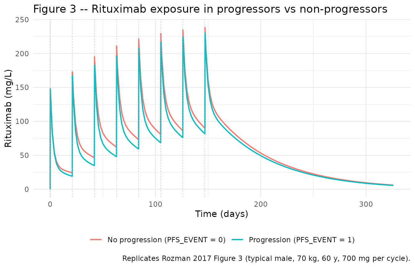
The progressor line (PFS_EVENT = 1, slower kdes = 0.0254 /day, half-life of CL2 decay 27.2 days) accumulates to higher trough concentrations than the non-progressor line (kdes = 0.143 /day, half-life of CL2 decay 4.85 days), matching the Rozman 2017 Figure 3 narrative: sustained target-mediated clearance in progressors gives higher total CL despite comparable baseline CL2,0, so the model initially predicts lower concentrations for progressors and only diverges once the non-progressor’s target-mediated clearance has decayed away.
Figure 3 (stochastic) – 90% prediction intervals
The paper’s Figure 3 shading is a 90% prediction interval from Monte-Carlo sampling of the random effects. Reproduced here with 200 subjects per arm, all carrying the same typical covariates so only the etas drive spread.
set.seed(20170132)

# Use nSub via rxSolve rather than pre-creating 200 rows in the event table.
# rxSolve replicates the single-subject event table across nSub subjects,
# resampling etas per subject.
events_stoch_np <- make_cohort("No progression", n = 1, WT = 70, AGE = 60,
                               SEXF = 0L, PFS_EVENT = 0L, id_offset = 0L)
events_stoch_p  <- make_cohort("Progression",    n = 1, WT = 70, AGE = 60,
                               SEXF = 0L, PFS_EVENT = 1L, id_offset = 1L)

sim_stoch_np <- rxode2::rxSolve(mod, events = events_stoch_np, nSub = 200,
                                keep = c("cohort", "PFS_EVENT")) |>
  as.data.frame()
sim_stoch_p  <- rxode2::rxSolve(mod, events = events_stoch_p,  nSub = 200,
                                keep = c("cohort", "PFS_EVENT")) |>
  as.data.frame()

sim_stoch <- bind_rows(sim_stoch_np, sim_stoch_p)

vpc <- sim_stoch |>
  filter(!is.na(Cc)) |>
  group_by(cohort, time) |>
  summarise(Q05 = quantile(Cc, 0.05, na.rm = TRUE),
            Q50 = quantile(Cc, 0.50, na.rm = TRUE),
            Q95 = quantile(Cc, 0.95, na.rm = TRUE),
            .groups = "drop")

ggplot(vpc, aes(x = time, colour = cohort, fill = cohort)) +
  geom_ribbon(aes(ymin = Q05, ymax = Q95), alpha = 0.2, colour = NA) +
  geom_line(aes(y = Q50), linewidth = 0.7) +
  geom_vline(xintercept = dose_times, colour = "grey70", linetype = "dashed",
             linewidth = 0.2) +
  labs(x = "Time (days)", y = "Rituximab (mg/L)",
       colour = NULL, fill = NULL,
       title = "Figure 3 -- 90% prediction intervals (200 subjects per arm)",
       caption = paste("Median (solid) and 5th/95th percentiles (shaded);",
                       "200 stochastic subjects per PFS_EVENT arm.")) +
  theme_minimal() +
  theme(legend.position = "bottom")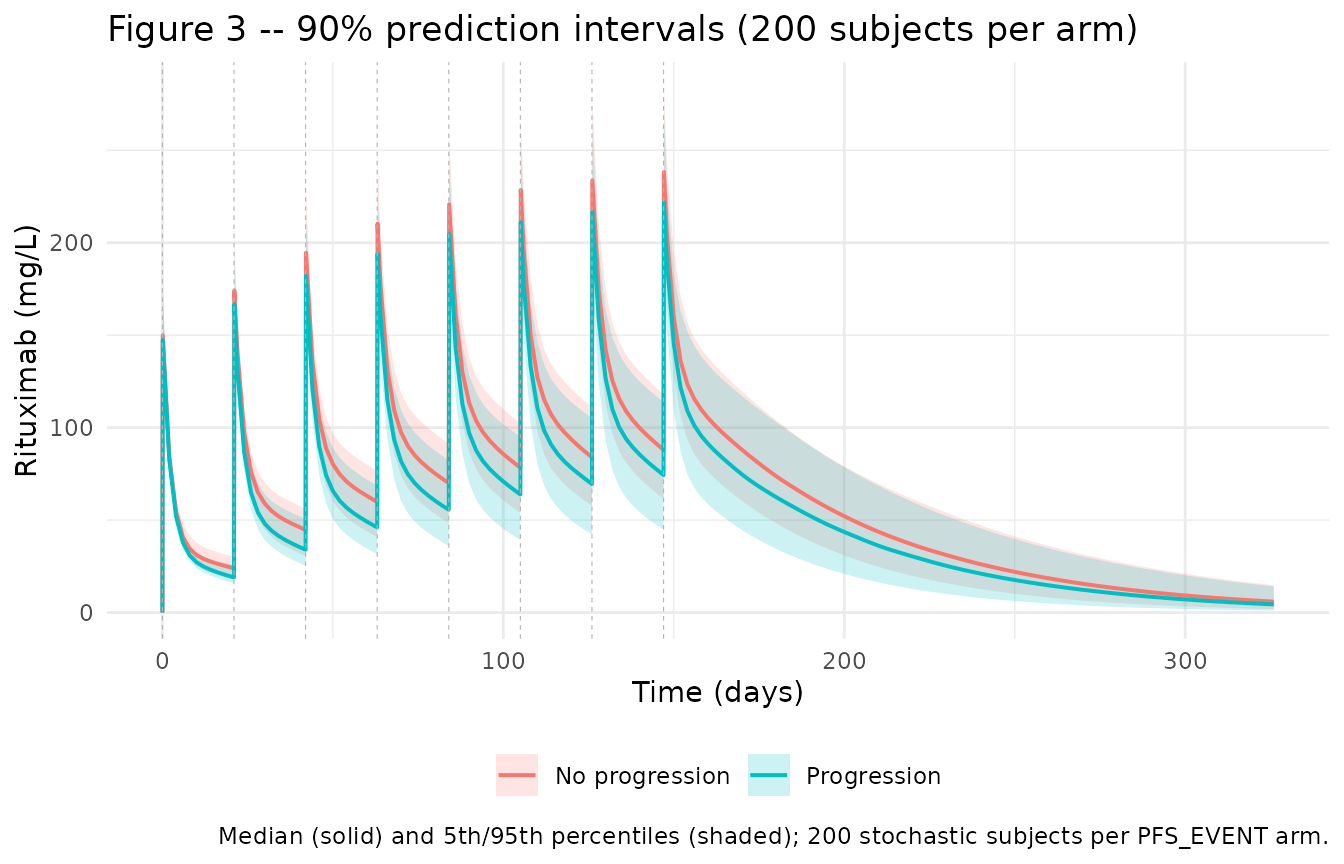
Prediction intervals are wide because Rozman 2017 reports very large IIV on KD (CV 161%, shrinkage 22.7%) – the paper’s Figure 3 shows similarly wide bands and cautions in the Discussion that the model’s precision on KD is limited by the modest sample size (n = 29).
PKNCA validation
Rozman 2017 reports observed rituximab trough serum levels (median [range]) during the R-CHOP treatment window: 23.2 (17.9-31.5) mg/L before the second infusion; 80.7 (50.0-129.4) mg/L before the last-cycle infusion (Results, “Rituximab serum levels”). These trough values are compared here against PKNCA-derived Cmin at the same trough time points from the typical-value simulation. Cmax and per-cycle AUC are also reported for completeness.
sim_nca_raw <- rxode2::rxSolve(mod_typical, events = events_fig3,
                               keep = c("cohort", "PFS_EVENT")) |>
  as.data.frame()
#> ℹ omega/sigma items treated as zero: 'etalcl_exp_inf', 'etalcl_exp_kdes', 'etalvc'
#> Warning: multi-subject simulation without without 'omega'

# One PKNCA interval per cycle (0-21 days, 21-42 days, ...). The last
# interval extends from the final dose (day 147) to 21 days past it (day
# 168) so a Cmin can be computed for the cycle-8 dosing interval.
cycle_intervals <- tibble(
  cycle   = seq_along(dose_times),
  start   = dose_times,
  end     = c(dose_times[-1], last_dose + 21),
  cmax    = TRUE,
  cmin    = TRUE,
  tmax    = TRUE,
  auclast = TRUE
)

# Retain concentration rows through end of the cycle-8 dosing window
# (day 168). Include a defensive t=0 row per (id, cohort) so PKNCA anchors
# every subject at time zero (Cc = 0 pre-dose since dosing is IV to central).
sim_nca <- sim_nca_raw |>
  filter(!is.na(Cc), time <= last_dose + 21) |>
  select(id, time, Cc, cohort)

sim_nca <- bind_rows(
  sim_nca,
  sim_nca |> distinct(id, cohort) |> mutate(time = 0, Cc = 0)
) |>
  distinct(id, cohort, time, .keep_all = TRUE) |>
  arrange(id, cohort, time)

dose_df <- events_fig3 |>
  filter(evid == 1) |>
  select(id, time, amt, cohort)

conc_obj <- PKNCA::PKNCAconc(sim_nca, Cc ~ time | cohort + id,
                             concu = "mg/L", timeu = "day")
dose_obj <- PKNCA::PKNCAdose(dose_df, amt ~ time | cohort + id,
                             doseu = "mg")

intervals <- cycle_intervals |> select(-cycle) |> as.data.frame()

nca_res <- PKNCA::pk.nca(PKNCA::PKNCAdata(conc_obj, dose_obj,
                                          intervals = intervals))

nca_wide <- as.data.frame(nca_res$result) |>
  select(cohort, start, end, PPTESTCD, PPORRES) |>
  tidyr::pivot_wider(names_from = PPTESTCD, values_from = PPORRES) |>
  left_join(cycle_intervals |> select(cycle, start, end), by = c("start", "end"))
Trough levels: simulated vs paper
Table 3 below compares simulated cmin at the end of each
dosing interval against the paper’s reported medians for
pre-second-infusion (cycle 1 -> cycle 2 trough) and pre-cycle-8
trough. The typical-value simulation is compared against the paper’s
median observed trough – a magnitude check on the drug-accumulation
prediction.
# Pre-second-infusion trough is at the end of cycle 1 (day 21); pre-cycle-8
# trough is at the end of cycle 7 (day 147).
troughs <- nca_wide |>
  filter(cycle %in% c(1, 7)) |>
  mutate(`Trough (cycle boundary)` = case_when(
    cycle == 1 ~ "Pre-cycle 2 (day 21)",
    cycle == 7 ~ "Pre-cycle 8 (day 147)"
  )) |>
  select(cohort, `Trough (cycle boundary)`, `Cmin simulated (mg/L)` = cmin)

published <- tribble(
  ~cohort,                            ~`Trough (cycle boundary)`,        ~`Median trough observed (mg/L, Rozman 2017)`,
  "No progression (PFS_EVENT = 0)",   "Pre-cycle 2 (day 21)",             23.2,
  "No progression (PFS_EVENT = 0)",   "Pre-cycle 8 (day 147)",            80.7,
  "Progression (PFS_EVENT = 1)",      "Pre-cycle 2 (day 21)",             23.2,
  "Progression (PFS_EVENT = 1)",      "Pre-cycle 8 (day 147)",            80.7
)

troughs |>
  left_join(published, by = c("cohort", "Trough (cycle boundary)")) |>
  knitr::kable(caption = paste("Simulated typical-value trough vs Rozman 2017",
                                "median observed troughs. The paper reports pooled",
                                "medians across all 29 patients (not stratified by",
                                "PFS_EVENT), so the same reference value is shown",
                                "against both simulated arms."),
digits = 2)| cohort | Trough (cycle boundary) | Cmin simulated (mg/L) | Median trough observed (mg/L, Rozman 2017) |
|---|---|---|---|
| No progression (PFS_EVENT = 0) | Pre-cycle 2 (day 21) | 0.00 | 23.2 |
| No progression (PFS_EVENT = 0) | Pre-cycle 8 (day 147) | 86.24 | 80.7 |
| Progression (PFS_EVENT = 1) | Pre-cycle 2 (day 21) | 0.00 | 23.2 |
| Progression (PFS_EVENT = 1) | Pre-cycle 8 (day 147) | 75.95 | 80.7 |
Per-cycle NCA summary
nca_wide |>
  select(cohort, cycle, start, end,
         `Cmax (mg/L)`     = cmax,
         `Cmin (mg/L)`     = cmin,
         `Tmax (day)`      = tmax,
         `AUClast (mg*day/L)` = auclast) |>
  arrange(cohort, cycle) |>
  knitr::kable(caption = paste("Simulated typical-value NCA parameters per",
                                "R-CHOP cycle (typical male, 70 kg, 60 y, 700 mg",
                                "per cycle). AUClast is over the current cycle's",
                                "21-day interval; cycle 8 extends 21 days past",
                                "the final dose."),
digits = 2)| cohort | cycle | start | end | Cmax (mg/L) | Cmin (mg/L) | Tmax (day) | AUClast (mg*day/L) |
|---|---|---|---|---|---|---|---|
| No progression (PFS_EVENT = 0) | 1 | 0 | 21 | 148.08 | 0.00 | 0.1 | 893.08 |
| No progression (PFS_EVENT = 0) | 2 | 21 | 42 | 172.98 | 24.36 | 0.1 | 1465.88 |
| No progression (PFS_EVENT = 0) | 3 | 42 | 63 | 195.17 | 46.57 | 0.1 | 1865.73 |
| No progression (PFS_EVENT = 0) | 4 | 63 | 84 | 210.86 | 62.28 | 0.1 | 2142.33 |
| No progression (PFS_EVENT = 0) | 5 | 84 | 105 | 221.81 | 73.25 | 0.1 | 2337.12 |
| No progression (PFS_EVENT = 0) | 6 | 105 | 126 | 229.45 | 80.90 | 0.1 | 2470.93 |
| No progression (PFS_EVENT = 0) | 7 | 126 | 147 | 234.77 | 86.24 | 0.1 | 2566.35 |
| No progression (PFS_EVENT = 0) | 8 | 147 | 168 | 238.49 | 89.96 | 0.1 | 2630.76 |
| Progression (PFS_EVENT = 1) | 1 | 0 | 21 | 148.07 | 0.00 | 0.1 | 818.64 |
| Progression (PFS_EVENT = 1) | 2 | 21 | 42 | 167.50 | 19.22 | 0.1 | 1220.14 |
| Progression (PFS_EVENT = 1) | 3 | 42 | 63 | 183.19 | 34.79 | 0.1 | 1548.69 |
| Progression (PFS_EVENT = 1) | 4 | 63 | 84 | 196.52 | 48.05 | 0.1 | 1820.18 |
| Progression (PFS_EVENT = 1) | 5 | 84 | 105 | 207.77 | 59.27 | 0.1 | 2045.47 |
| Progression (PFS_EVENT = 1) | 6 | 105 | 126 | 217.04 | 68.52 | 0.1 | 2224.68 |
| Progression (PFS_EVENT = 1) | 7 | 126 | 147 | 224.47 | 75.95 | 0.1 | 2367.74 |
| Progression (PFS_EVENT = 1) | 8 | 147 | 168 | 230.29 | 81.76 | 0.1 | 2475.79 |
The progressor arm’s slower target-mediated CL decay yields higher-than-typical AUC and Cmin in later cycles, consistent with the paper’s headline finding that patients with disease progression have higher rituximab exposure through R-CHOP.
Assumptions and deviations
-
Progression indicator is post-hoc (selection-bias
caveat).
PFS_EVENTis assigned from longitudinal response-assessment data (per the revised response criteria for malignant lymphoma) at end of follow-up, and Rozman 2017 uses it as a covariate on the PK parametercl_exp_kdesin the same analysis. This is unusual – a PK covariate is normally a baseline pre-treatment characteristic – but is what the paper did (Rozman 2017 Methods, “Covariate model”, and Results, “Of all covariate relationships tested, we observed a significant association … KD with disease progression”). Using an outcome as a covariate carries selection-bias implications for prospective PK prediction (a subject’sPFS_EVENTvalue is not known at treatment start), so downstream users simulating exposure in individuals with unknown future progression status should typically usePFS_EVENT = 0(the reference stratum) or draw the indicator from the observed 20.7% event rate. -
Canonical column name
PFS_EVENT(introduced by this paper). The paper’s prose descriptor “disease progression” is registered ininst/references/covariate-columns.mdunder the standard oncology- trial namePFS_EVENT(progression-free-survival event indicator). Rozman 2017 does not disclose the NONMEM$INPUTcolumn name; the canonical follows the widely used PFS-event convention rather than a Rozman-specific abbreviation. -
Reference weight 70 kg, reference age 60 years, male
reference for V1, PFS_EVENT = 0 reference for KD. These are the
four anchors of the typical-value predictions in Rozman 2017 Table 2 and
are directly supported by the paper’s simulation baseline for Figure 3
(“typical male patient, 70 kg body weight, age 60 years”) and the
reported progressor-vs-non-progressor KD split. The age-effect equation
is linear in
(AGE - 60); the weight effect is a power in(WT / 70)^1.23. The 95% CI on the WT exponent (0.70-1.73) brackets the theoretical allometric value 0.75 (Rozman 2017 Results, paragraph following Equation 3). - Infusion regimen simplified to 1.5-h IV infusion per cycle. Rozman 2017 dosed cycle 1 as a slow ramp (50 mg/h ramped by 50 mg/h every 30 min to a maximum of 400 mg/h; ~2-3 h for 700 mg) and cycles 2-8 as a fast infusion (20% of dose over 30 min plus 80% over 60 min; ~1.5 h for 700 mg). The vignette uses a uniform 1.5-h IV infusion for visual clarity. Rituximab has slow disposition (terminal half-life weeks), so the ~30-90 minute difference in infusion duration is negligible for the trough / Cmin / AUC comparisons plotted here.
- No inter-occasion variability (IOV). Rozman 2017 estimated variability on CL1, KD, and V1 as inter-individual only; no IOV was fit (Methods, “Covariate model”: IIV is described by exponential random effect model with no per-cycle decomposition). Downstream users wanting cycle-to-cycle variability should add an occasion indicator and a per-occasion eta.
- Very large IIV on KD (CV 161%). The paper’s own Table 2 reports 22.7% shrinkage on the KD random effect and 95% CI 0.0478-0.418 for the typical KD (approximately a 10-fold range). Predictions of the time-varying CL arm therefore carry very wide uncertainty even at the reference-subject values used in Figure 3.
- Residual error is on the linear concentration scale (additive + proportional). Rozman 2017 selected a combined additive + proportional error model (Methods, “Structural model development”): 2.46 mg/L additive plus 15.9% proportional. The additive term dominates at trough concentrations (~2-3 mg/L relative to observed troughs of 20-80 mg/L, i.e. 3-12% relative contribution); the proportional term dominates at peaks.
- Population 100% Caucasian. Rozman 2017 was conducted at a single Slovenian centre; ethnicity distribution outside Caucasian populations was not evaluated. Extrapolation to other populations should note this limitation.
- Trough comparison uses paper’s pooled median (not stratified by PFS_EVENT). Rozman 2017 reports median trough levels across all 29 patients (Results, “Rituximab serum levels”: 23.2 mg/L median pre- cycle-2 trough; 80.7 mg/L median pre-cycle-8 trough) without stratifying by progression status. The reference value in the trough-comparison table is therefore identical across the two simulated arms; the paper reports the progressor / non-progressor split only as time-varying CL half-lives (27.2 days vs 4.85 days), not as observed-trough medians.