Fosfomycin plasma and prostate PK (Cojutti 2026)
Source:vignettes/articles/Cojutti_2026_fosfomycin.Rmd
Cojutti_2026_fosfomycin.RmdModel and source
mod <- rxode2::rxode2(readModelDb("Cojutti_2026_fosfomycin"))
#> ℹ parameter labels from comments will be replaced by 'label()'- Citation: Cojutti PG, Berrino PM, Rotaru V, Bianchi L, Schiavina R, Brunocilla E, Viale P, Pea F. Population Pharmacokinetics of a Novel Oral Fosfomycin Prophylactic Scheme in the Plasma and Prostate of Patients Undergoing Endoscopic Surgery for Benign Prostatic Hyperplasia. Clin Pharmacokinet. 2026;65:109-118. doi:10.1007/s40262-025-01586-1.
- Article: https://doi.org/10.1007/s40262-025-01586-1
- Description: One-compartment population PK model with first-order absorption for oral fosfomycin trometamol in plasma, joined to prostate tissue by a direct- response power function (Cprostate = PR * Cc^POW), in 104 men undergoing endoscopic surgery (HoLEP or TURP) for benign prostatic hyperplasia after a prophylactic scheme of two 3 g oral doses 12 h apart. Prostate concentration is algebraic in the plasma concentration; there is no prostate ODE state. Clearance and volume are apparent (CL/F, V/F); ka and its IIV are fixed. V/F carries an exponential effect of uncentred body weight. Constant (additive) residual error on both outputs (Cojutti 2026).
Cojutti 2026 fitted plasma and prostate-tissue fosfomycin concentrations jointly in Monolix 2023R1. Plasma is a one-compartment model with first-order absorption. Prostate tissue is linked to plasma by a direct-response power function, so the prostate concentration is an algebraic function of the plasma concentration and has no ODE state of its own:
Twelve candidate structures were compared (one or two compartments; a
proportional, power or saturable link; ka estimated or
fixed). The selected structure is model 5 of the paper’s Table S1
(electronic supplementary material, ESM): one compartment, a power link,
and ka fixed. The ESM supplies the final Monolix code,
whose EQUATION: block is the source for both equations in
the model file:
Cc = pkmodel(ka, V, Cl)
Cp = PR*(Cc^POW)
Population
104 men undergoing endoscopic surgery for benign prostatic hyperplasia at a single Italian centre (Bologna, February 2022 to September 2023). 85 (81.7%) had Holmium laser enucleation of the prostate and 19 (18.3%) had transurethral resection. Median (range): age 70 (49-84) years, weight 78 (60-107) kg, BMI 26.3 (20.6-41.5) kg/m^2, CKD-EPI eGFR 78.5 (34-102) mL/min/1.73 m^2, prostate volume 75 (20-220) mL, PSA 3.10 (0.02-66) ng/mL (Results, first paragraph).
Every patient took oral fosfomycin trometamol 3 g 12 h before the end
of the prophylactic scheme and 3 g at its end (t = -12 h
and t = 0 h). Each contributed exactly one plasma sample
and one concomitant prostate biopsy, at a median of 3.86 (0.42-10.7) h
after the second dose. There were no samples during absorption, which is
why ka and its variability had to be fixed.
str(mod$population)
#> List of 13
#>  $ species       : chr "human"
#>  $ n_subjects    : int 104
#>  $ n_studies     : int 1
#>  $ n_observations: int 208
#>  $ age_range     : chr "49-84 years (median 70)"
#>  $ weight_range  : chr "60-107 kg (median 78)"
#>  $ sex_female_pct: num 0
#>  $ race_ethnicity: chr "not reported"
#>  $ disease_state : chr "Men with benign prostatic hyperplasia undergoing endoscopic surgery: Holmium laser enucleation of the prostate "| __truncated__
#>  $ renal_function: chr "CKD-EPI eGFR median 78.5 (34-102) mL/min/1.73 m^2; 98% (102/104) above 50 mL/min."
#>  $ dose_range    : chr "Oral fosfomycin trometamol 3 g twice, 12 h apart, the second dose given before surgery (3 g at t = -12 h and 3 "| __truncated__
#>  $ regions       : chr "Italy (single centre: IRCCS Azienda Ospedaliero-Universitaria di Bologna)"
#>  $ notes         : chr "One plasma sample and one concomitant prostate biopsy per patient, at a median of 3.86 (0.42-10.7) h after the "| __truncated__
Source trace
| Model element | Value | Source location |
|---|---|---|
lka (ka, 1/h) |
0.92, fixed | Table 1; Methods 2.2 (value from healthy volunteers, ref. 23) |
lcl (CL/F, L/h) |
14.68 (RSE 14.4%) | Table 1 |
lvc (V/F at 0 kg, L) |
60.86 (RSE 44.1%) | Table 1; Results equation
V = 60.86 x e^(0.02 x BW)
|
e_wt_vc (1/kg) |
0.02 (RSE 26.9%) | Table 1, beta_V_weight
|
lrprostate (PR) |
0.26 (RSE 7.09%) | Table 1; footnote “penetration ratio at a plasma concentration of 1 mg/L” |
lpow_prostate (POW) |
1.57 (RSE 1.80%) | Table 1 |
etalka |
SD 1.09, fixed | Table 1, omega_ka
|
etalcl |
SD 0.76 (CV 87.86%) | Table 1, omega_CL; CV from ESM Table S3 |
etalvc |
SD 0.38 (CV 39.52%) | Table 1, omega_V; ESM Table S3 |
etalrprostate |
SD 0.42 (CV 44.27%) | Table 1, omega_PR; ESM Table S3 |
etalpow_prostate |
SD 0.095 (CV 9.5%) | Table 1, omega_POW; ESM Table S3 |
addSd (mg/L) |
1.35 (RSE 20.5%) | Table 1, a_plasma (constant error) |
addSd_Cprostate (ug/g) |
1.01 (RSE 34.0%) | Table 1, a_prostate (constant error) |
| One-compartment first-order absorption | – | ESM model code, Cc = pkmodel(ka, V, Cl)
|
| Weight on V/F | V = 60.86 * exp(0.02 * WT) |
Results, “Model equations” |
| Prostate link | Cprostate = PR * Cc^POW |
Methods 2.2 model (2); Results Cp = 0.26 x Cc^1.57; ESM
model code |
Table 1 lists the random effects as standard
deviations on the log scale. The ESM Table S3 prints a CV
column next to each one, and that column matches
sqrt(exp(omega^2) - 1) to the rounding of the printed SDs,
which confirms they are SDs rather than variances. The model file
therefore squares each value.
omega <- c(ka = 1.09, V = 0.38, CL = 0.76, PR = 0.42, POW = 0.095)
# Half a unit in the last printed decimal of each SD.
half_ulp <- c(ka = 0.005, V = 0.005, CL = 0.005, PR = 0.005, POW = 0.0005)
cv_published <- c(ka = 151.02, V = 39.52, CL = 87.86, PR = 44.27, POW = 9.5)
# The CV column was computed from the unrounded SDs, so invert it and check
# that the result rounds to the printed SD. Read as variances instead, the
# same CVs would need omega = 1.19, 0.15, 0.57, 0.18 and 0.009.
sd_from_cv <- sqrt(log(1 + (cv_published / 100)^2))
knitr::kable(
  data.frame(omega_SD = omega, CV_published = cv_published, SD_from_CV = sd_from_cv) |>
    dplyr::rename("omega, Table 1 (SD)" = omega_SD, "CV, ESM Table S3 (%)" = CV_published, "sqrt(log(1 + CV^2))" = SD_from_CV),
  digits = 4
)| omega, Table 1 (SD) | CV, ESM Table S3 (%) | sqrt(log(1 + CV^2)) | |
|---|---|---|---|
| ka | 1.090 | 151.02 | 1.0900 |
| V | 0.380 | 39.52 | 0.3810 |
| CL | 0.760 | 87.86 | 0.7564 |
| PR | 0.420 | 44.27 | 0.4230 |
| POW | 0.095 | 9.50 | 0.0948 |
The printed equations reproduce the paper’s own medians
The volume equation uses absolute body weight with no centring, so the typical value of 60.86 L applies to a 0 kg patient. Evaluated at the cohort’s median weight of 78 kg, it gives the paper’s separately reported median individual apparent volume of 288.9 L. That agreement confirms the exponential form on uncentred weight. The Methods text calls the covariate model “a power function”, but a power model, or a model centred on the median, would put the typical V/F at 60.86 L.
The link function evaluated at the observed median plasma concentration (11.1 mg/L) gives a prostate concentration close to the observed median (11.6 ug/g). The implied ratio of 1.03 is close to the reported median observed prostate-to-plasma ratio of 1.04.
v_at_median_wt <- 60.86 * exp(0.02 * 78)
cp_at_median_cc <- 0.26 * 11.1^1.57
knitr::kable(tibble::tribble(
  ~Quantity, ~Published, ~Model,
  "Median individual V/F at 78 kg (L)", 288.9, v_at_median_wt,
  "Prostate conc. at plasma 11.1 mg/L (ug/g)", 11.6, cp_at_median_cc,
  "Prostate/plasma ratio at plasma 11.1 mg/L", 1.04, cp_at_median_cc / 11.1
), digits = 2)| Quantity | Published | Model |
|---|---|---|
| Median individual V/F at 78 kg (L) | 288.90 | 289.62 |
| Prostate conc. at plasma 11.1 mg/L (ug/g) | 11.60 | 11.38 |
| Prostate/plasma ratio at plasma 11.1 mg/L | 1.04 | 1.03 |
Mass balance under typical values
CL and V are apparent oral parameters (F = 1), so after a single 3 g dose the typical-value plasma AUC(0-inf) must equal Dose / CL = 3000 / 14.68 = 204.4 mg h/L, whatever the body weight. Both sides use the same typical parameters, so the difference is pure numerical error and a tight bound is appropriate. The check also confirms that the two ODE states are the two named compartments in order.
# The model declares two residual-error endpoints (Cc and Cprostate), so every
# observation row must nominate one: observation rows sit on the central
# state with dvid = 1. Both Cc and Cprostate are returned as columns at every
# observation time whichever endpoint is nominated.
# useLinCmt = FALSE keeps the explicit ODEs rather than an analytic solution.
t_single <- sort(unique(c(seq(0, 2, by = 0.02), seq(2, 24, by = 0.1), seq(24, 300, by = 1))))
ev_single <- dplyr::bind_rows(
  data.frame(id = 1L, time = 0, amt = 3000, evid = 1L, cmt = "depot", dvid = NA_integer_),
  data.frame(id = 1L, time = t_single, amt = 0, evid = 0L, cmt = "central", dvid = 1L)
)
typ <- rxode2::rxSolve(
  rxode2::zeroRe(mod), ev_single,
  params = c(WT = 78), useLinCmt = FALSE
) |> as.data.frame()
#> ℹ omega/sigma items treated as zero: 'etalka', 'etalcl', 'etalvc', 'etalrprostate', 'etalpow_prostate'

stopifnot(identical(mod$state, c("depot", "central")))
# The prostate output is exactly the power link of the plasma output.
stopifnot(isTRUE(all.equal(typ$Cprostate, 0.26 * typ$Cc^1.57, tolerance = 1e-8)))

nca_typ <- PKNCA::PKNCAdata(
  PKNCA::PKNCAconc(typ |> dplyr::mutate(id = 1L) |> dplyr::select(id, time, Cc), Cc ~ time | id),
  PKNCA::PKNCAdose(data.frame(id = 1L, time = 0, amt = 3000), amt ~ time | id),
  intervals = data.frame(start = 0, end = Inf, aucinf.obs = TRUE, cmax = TRUE, tmax = TRUE, half.life = TRUE)
) |>
  PKNCA::pk.nca() |>
  as.data.frame()
auc_typ <- nca_typ$PPORRES[nca_typ$PPTESTCD == "aucinf.obs"]
c(AUCinf = auc_typ, Dose_over_CL = 3000 / 14.68)
#>       AUCinf Dose_over_CL
#>     204.3581     204.3597
stopifnot(abs(auc_typ / (3000 / 14.68) - 1) < 0.005)
Virtual cohort
The paper reports body weight only as a median and range (78, 60-107 kg). Weight is drawn from a log-normal centred on 78 kg, and draws outside the observed range are rejected and redrawn rather than clamped to it, so that the cohort’s median is not distorted. The same weights are reused for all three dosing schemes of the paper’s Monte Carlo simulation (Methods 2.4):
-
A: 3 g at
t = -12 hand 3 g att = 0 h(the studied scheme); -
B: 3 g at
t = -12 hand 6 g att = 0 h; -
C: 3 g at
t = -8 hand 6 g att = 0 h.
In the event tables the first dose is at time 0, so
t = 0 h of the paper is time 12 here.
set.seed(2026)
rxode2::rxSetSeed(2026)
n_per_arm <- 200L

draw_wt <- function(n, median_wt = 78, sdlog = 0.14, lower = 60, upper = 107) {
  out <- numeric(0)
  while (length(out) < n) {
    x <- stats::rlnorm(2L * n, log(median_wt), sdlog)
    out <- c(out, x[x >= lower & x <= upper])
  }
  out[seq_len(n)]
}
wt <- draw_wt(n_per_arm)

schemes <- tibble::tribble(
  ~scheme, ~t_first, ~amt_first, ~amt_second,
  "A: 3 g t-12h + 3 g t0h", 0, 3000, 3000,
  "B: 3 g t-12h + 6 g t0h", 0, 3000, 6000,
  "C: 3 g t-8h + 6 g t0h", 4, 3000, 6000
)

obs_grid <- sort(unique(c(seq(0, 12, by = 0.25), seq(12, 24, by = 0.05))))

make_arm <- function(k) {
  s <- schemes[k, ]
  ids <- (k - 1L) * n_per_arm + seq_len(n_per_arm)
  doses <- tidyr::expand_grid(id = ids, dose_no = 1:2) |>
    dplyr::mutate(
      time = ifelse(dose_no == 1, s$t_first, 12),
      amt = ifelse(dose_no == 1, s$amt_first, s$amt_second),
      evid = 1L, cmt = "depot", dvid = NA_integer_
    ) |>
    dplyr::select(-dose_no)
  obs <- tidyr::expand_grid(id = ids, time = obs_grid) |>
    dplyr::mutate(amt = 0, evid = 0L, cmt = "central", dvid = 1L)
  dplyr::bind_rows(doses, obs) |>
    dplyr::mutate(scheme = s$scheme, WT = wt[id - (k - 1L) * n_per_arm]) |>
    dplyr::arrange(id, time, dplyr::desc(evid))
}
events <- dplyr::bind_rows(lapply(seq_len(nrow(schemes)), make_arm))
stopifnot(
  anyDuplicated(events[, c("id", "time", "evid")]) == 0L,
  dplyr::n_distinct(events$id) == 3L * n_per_arm
)
summary(wt)
#>    Min. 1st Qu.  Median    Mean 3rd Qu.    Max.
#>   60.13   70.64   77.89   78.72   84.79  105.85
Simulation
sim <- rxode2::rxSolve(mod, events, keep = c("scheme", "WT"), useLinCmt = FALSE) |>
  as.data.frame() |>
  dplyr::mutate(tad2 = time - 12)
The paper reports the median of the individual (post hoc) apparent V and CL as 288.9 L and 15.7 L/h. The simulated cohort’s medians should be close. They are not identical: the post hoc estimates are shrunk towards the typical values, and the simulated weights only reproduce the cohort’s median and range. With a CL/F variability of SD 0.76 the median of 200 subjects carries a standard error of about 7%, so the bound is 25%; a mis-transcribed CL or V moves the median by far more.
indiv <- sim |>
  dplyr::filter(grepl("^A", scheme)) |>
  dplyr::distinct(id, vc, cl)
med_check <- tibble::tribble(
  ~Parameter, ~Published, ~Simulated,
  "Median individual V/F (L)", 288.9, stats::median(indiv$vc),
  "Median individual CL/F (L/h)", 15.7, stats::median(indiv$cl)
) |>
  dplyr::mutate(`Difference (%)` = 100 * (Simulated / Published - 1))
knitr::kable(med_check, digits = 1)| Parameter | Published | Simulated | Difference (%) |
|---|---|---|---|
| Median individual V/F (L) | 288.9 | 294.2 | 1.8 |
| Median individual CL/F (L/h) | 15.7 | 15.2 | -3.5 |
Replicate published figures
Figure 2: plasma and prostate profiles for the studied scheme
sim |>
  dplyr::filter(grepl("^A", scheme)) |>
  tidyr::pivot_longer(c(Cc, Cprostate), names_to = "matrix", values_to = "conc") |>
  dplyr::mutate(matrix = dplyr::recode(matrix, Cc = "Plasma (mg/L)", Cprostate = "Prostate (ug/g)")) |>
  dplyr::group_by(matrix, tad2) |>
  dplyr::summarise(
    q05 = stats::quantile(conc, 0.05), q50 = stats::median(conc), q95 = stats::quantile(conc, 0.95),
    .groups = "drop"
  ) |>
  ggplot(aes(tad2, q50, colour = matrix, fill = matrix)) +
  geom_ribbon(aes(ymin = q05, ymax = q95), alpha = 0.2, colour = NA) +
  geom_line(linewidth = 0.8) +
  scale_colour_manual(values = c("firebrick", "goldenrod")) +
  scale_fill_manual(values = c("firebrick", "goldenrod")) +
  labs(x = "Time relative to the second dose (h)", y = "Fosfomycin concentration", colour = NULL, fill = NULL) +
  theme_bw()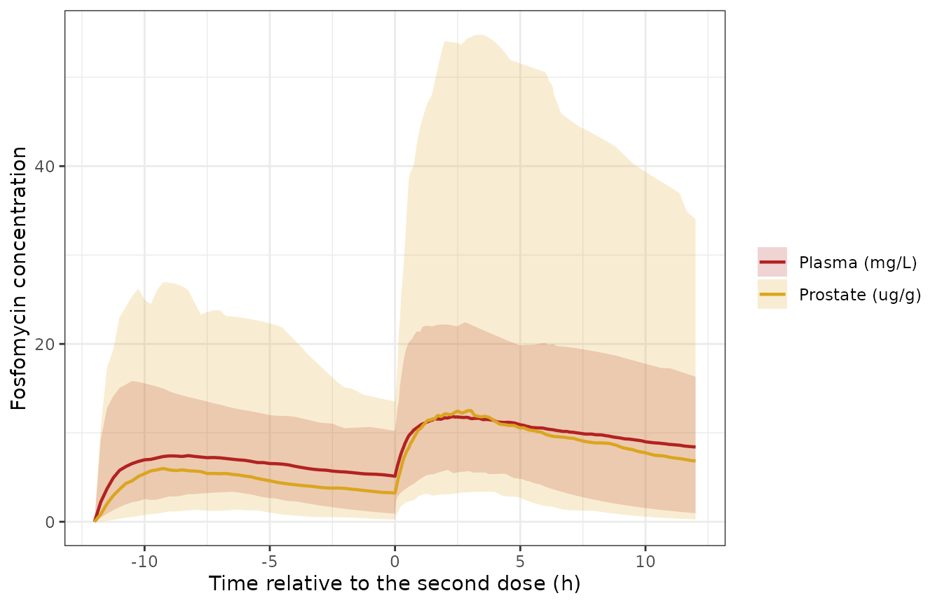
Replicates Figure 2 of Cojutti 2026: simulated fosfomycin plasma (mg/L) and prostate (ug/g) concentrations after 3 g at t = -12 h and 3 g at t = 0 h. Lines are medians; ribbons are 5th-95th percentiles.
Figure 3: prostate-to-plasma penetration ratio
Figure 3 is a histogram of the simulated penetration ratio
(Cprostate / Cc) for the studied scheme. The text reports
the share of simulated subjects in three bins. The time at which the
ratio is evaluated is not stated, so it is taken here at the study’s
median sampling time (the 3.85 h grid point, nearest to the 3.86 h
median after the second dose). Under the power link the ratio is
PR * Cc^(POW - 1), so it rises with the plasma
concentration. A wrong POW or PR therefore
moves all three bins together. With 200 subjects the binomial standard
error of each share is about 3.5 percentage points, so the tolerance is
12 percentage points.
ratio_df <- sim |>
  dplyr::filter(grepl("^A", scheme), abs(tad2 - 3.85) < 1e-6) |>
  dplyr::mutate(ratio = Cprostate / Cc)
stopifnot(nrow(ratio_df) == n_per_arm)

ratio_bins <- tibble::tibble(
  Bin = c("< 1", "1 - 2", "> 2"),
  Published = c(48.3, 37.5, 14.2),
  Simulated = 100 * c(
    mean(ratio_df$ratio < 1),
    mean(ratio_df$ratio >= 1 & ratio_df$ratio <= 2),
    mean(ratio_df$ratio > 2)
  )
)
knitr::kable(ratio_bins |> dplyr::rename("Penetration ratio" = Bin, "Published (%)" = Published, "Simulated (%)" = Simulated), digits = 1)| Penetration ratio | Published (%) | Simulated (%) |
|---|---|---|
| < 1 | 48.3 | 48 |
| 1 - 2 | 37.5 | 38 |
| > 2 | 14.2 | 14 |
stopifnot(all(abs(ratio_bins$Simulated - ratio_bins$Published) < 12))

ggplot(ratio_df, aes(ratio)) +
  geom_histogram(binwidth = 0.25, boundary = 0, fill = "grey60", colour = "white") +
  geom_vline(xintercept = c(1, 2), linetype = "dashed") +
  labs(x = "Prostate-to-plasma penetration ratio", y = "Simulated subjects") +
  theme_bw()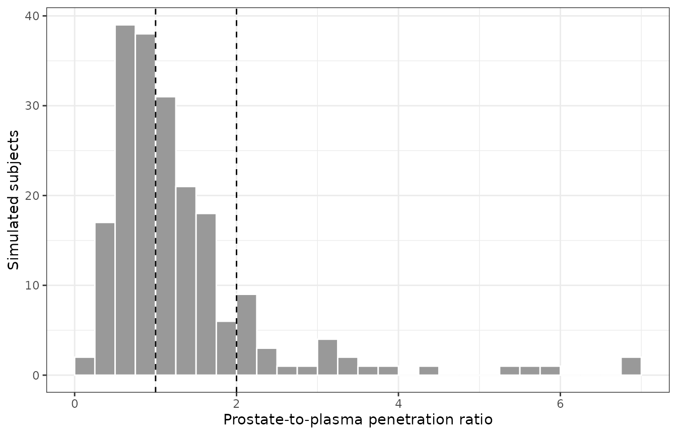
Replicates Figure 3 of Cojutti 2026: distribution of the simulated prostate-to-plasma penetration ratio, 3.86 h after the second 3 g dose.
PKNCA validation
The paper reports no NCA table. PKNCA is used here to compute each subject’s plasma and prostate exposure over the 12 h vulnerable period after the second dose (time 12-24 in the event tables), grouped by dosing scheme. The plasma AUC over that window drives the probability of target attainment (PTA) below.
nca_input <- function(df, conc_col) {
  out <- df |>
    dplyr::filter(!is.na(.data[[conc_col]])) |>
    dplyr::select(id, time, scheme, conc = dplyr::all_of(conc_col))
  # Guarantee a pre-dose time-zero row per subject (extravascular, so 0).
  dplyr::bind_rows(out, out |> dplyr::distinct(id, scheme) |> dplyr::mutate(time = 0, conc = 0)) |>
    dplyr::distinct(id, scheme, time, .keep_all = TRUE) |>
    dplyr::arrange(scheme, id, time)
}
dose_df <- events |>
  dplyr::filter(evid == 1) |>
  dplyr::select(id, time, amt, scheme)
intervals_vp <- data.frame(start = 12, end = 24, cmax = TRUE, tmax = TRUE, auclast = TRUE)

run_nca <- function(conc_col) {
  PKNCA::PKNCAdata(
    PKNCA::PKNCAconc(nca_input(sim, conc_col), conc ~ time | scheme + id),
    PKNCA::PKNCAdose(dose_df, amt ~ time | scheme + id),
    intervals = intervals_vp
  ) |>
    PKNCA::pk.nca() |>
    as.data.frame() |>
    dplyr::mutate(matrix = conc_col)
}
nca_res <- dplyr::bind_rows(run_nca("Cc"), run_nca("Cprostate"))

nca_res |>
  dplyr::group_by(matrix, scheme, PPTESTCD) |>
  dplyr::summarise(median = stats::median(PPORRES), .groups = "drop") |>
  tidyr::pivot_wider(names_from = PPTESTCD, values_from = median) |>
  dplyr::rename(
    "Matrix" = matrix, "Scheme" = scheme,
    "AUC 0-12 h after dose 2" = auclast, "Cmax" = cmax, "Tmax after dose 2 (h)" = tmax
  ) |>
knitr::kable(digits = 2)| Matrix | Scheme | AUC 0-12 h after dose 2 | Cmax | Tmax after dose 2 (h) |
|---|---|---|---|---|
| Cc | A: 3 g t-12h + 3 g t0h | 118.11 | 12.33 | 2.75 |
| Cc | B: 3 g t-12h + 6 g t0h | 191.39 | 19.76 | 3.47 |
| Cc | C: 3 g t-8h + 6 g t0h | 201.91 | 21.65 | 2.70 |
| Cprostate | A: 3 g t-12h + 3 g t0h | 113.78 | 13.76 | 2.75 |
| Cprostate | B: 3 g t-12h + 6 g t0h | 258.20 | 29.61 | 3.47 |
| Cprostate | C: 3 g t-8h + 6 g t0h | 255.49 | 28.21 | 2.70 |
Figure 4A: PTA of AUC/MIC > 83.3
Methods 2.4 defines the AUC target on the plasma concentration-time curve, over the 12 h vulnerable period after the second dose. The paper states that the PTA was optimal (at least 90%) up to an MIC of 0.5 mg/L for scheme A, and up to 1 mg/L for schemes B and C. A PTA of at least 90% at a given MIC is the same as the 10th percentile of AUC exceeding 83.3 x MIC. Each statement therefore brackets that percentile within a factor of two. The paper simulated 1000 subjects per scheme and this vignette 200, and the 10th percentile of 200 subjects carries a sampling error of about 10%, so each bound is relaxed by 25%:
-
A:
83.3 x 0.5 < P10(AUC) < 83.3 x 1; -
B and C:
83.3 x 1 < P10(AUC) < 83.3 x 2.
A robust quantile is checked rather than the PTA percentage, because a threshold-crossing percentage changes abruptly near the threshold.
auc_vp <- nca_res |>
  dplyr::filter(matrix == "Cc", PPTESTCD == "auclast") |>
  dplyr::select(id, scheme, auc = PPORRES)

pta_bracket <- auc_vp |>
  dplyr::group_by(scheme) |>
  dplyr::summarise(p10_auc = stats::quantile(auc, 0.1), .groups = "drop") |>
  dplyr::mutate(
    optimal_mic_published = ifelse(grepl("^A", scheme), 0.5, 1),
    lower = 83.3 * optimal_mic_published,
    upper = 83.3 * 2 * optimal_mic_published
  )
knitr::kable(
  pta_bracket |>
    dplyr::rename(
      "Scheme" = scheme, "P10 plasma AUC (mg h/L)" = p10_auc,
      "Highest optimal MIC, published (mg/L)" = optimal_mic_published,
      "Required P10 lower bound" = lower, "Required P10 upper bound" = upper
    ),
  digits = 1
)| Scheme | P10 plasma AUC (mg h/L) | Highest optimal MIC, published (mg/L) | Required P10 lower bound | Required P10 upper bound |
|---|---|---|---|---|
| A: 3 g t-12h + 3 g t0h | 60.5 | 0.5 | 41.6 | 83.3 |
| B: 3 g t-12h + 6 g t0h | 98.4 | 1.0 | 83.3 | 166.6 |
| C: 3 g t-8h + 6 g t0h | 121.8 | 1.0 | 83.3 | 166.6 |
stopifnot(all(pta_bracket$p10_auc > pta_bracket$lower / 1.25 & pta_bracket$p10_auc < pta_bracket$upper * 1.25))

mics <- 2^seq(-4, 4)
tidyr::expand_grid(auc_vp, mic = mics) |>
  dplyr::group_by(scheme, mic) |>
  dplyr::summarise(pta = 100 * mean(auc / mic > 83.3), .groups = "drop") |>
  ggplot(aes(mic, pta, colour = scheme)) +
  geom_line() +
  geom_point() +
  geom_hline(yintercept = 90, linetype = "dotted") +
  scale_x_continuous(trans = "log2", breaks = mics, labels = format(mics, drop0trailing = TRUE)) +
  labs(x = "MIC (mg/L)", y = "PTA (%)", colour = NULL) +
  theme_bw() +
  theme(legend.position = "bottom")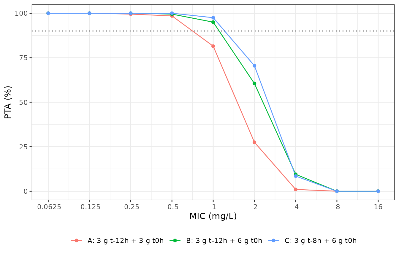
Replicates Figure 4A of Cojutti 2026: probability of attaining a plasma AUC(0-12 h after the second dose)/MIC above 83.3, by dosing scheme. The dotted line marks the 90% optimality threshold.
Figure 4B-D: 70% time above MIC in the prostate
For scheme A the paper reports optimal PTAs of 70% time above the MIC in prostate tissue for the whole 12 h vulnerable period against MICs up to 1 mg/L, and for only part of it (2-5 h) against MICs up to 4 mg/L. The simulation is consistent with both statements: the PTA over the whole window is at least 90% at 1 mg/L and below 90% at 4 mg/L, and both are asserted. The figure resolves the PTA over time; the 2-5 h sub-window is not checked.
ft_pta <- sim |>
  dplyr::filter(tad2 >= 0, tad2 <= 12) |>
  tidyr::expand_grid(mic = c(0.5, 1, 2, 4, 8)) |>
  dplyr::group_by(scheme, id, mic) |>
  dplyr::summarise(ft = mean(Cprostate > mic), .groups = "drop") |>
  dplyr::group_by(scheme, mic) |>
  dplyr::summarise(pta = 100 * mean(ft >= 0.7), .groups = "drop")
pta_a <- ft_pta |> dplyr::filter(grepl("^A", scheme))
stopifnot(
  pta_a$pta[pta_a$mic == 1] >= 90,
  pta_a$pta[pta_a$mic == 4] < 90
)
ft_pta |>
  tidyr::pivot_wider(names_from = mic, values_from = pta, names_prefix = "MIC ") |>
  dplyr::rename("Scheme" = scheme) |>
knitr::kable(digits = 1, caption = "PTA (%) of 70% time above MIC in prostate tissue over the 12 h after the second dose.")| Scheme | MIC 0.5 | MIC 1 | MIC 2 | MIC 4 | MIC 8 |
|---|---|---|---|---|---|
| A: 3 g t-12h + 3 g t0h | 97.0 | 95 | 90.0 | 75.0 | 51.0 |
| B: 3 g t-12h + 6 g t0h | 99.5 | 98 | 96.5 | 89.5 | 78.5 |
| C: 3 g t-8h + 6 g t0h | 99.0 | 98 | 97.0 | 92.5 | 79.5 |
Assumptions and deviations
-
New parameter names.
PRandPOWare carried aslrprostateandlpow_prostate. These are the prostate members of therelf/pow_elffamily used for the same power-function direct-response link to epithelial lining fluid (Dimelow 2018 avibactam). -
The Monolix model header is library boilerplate.
The
DESCRIPTION:block of the ESM model code says “administration is via a bolus” and “the PD model is a direct Emax model”. Both statements are contradicted by theEQUATION:block directly beneath them, which usespkmodel(ka, V, Cl)and a power link with no Emax or EC50. The equations were followed. - Covariate form. The Methods text describes the covariate model as “a power function”. The printed final equation is exponential on uncentred body weight, and only the exponential form reproduces the reported median individual V/F (see above). The equation was followed.
-
Table 1 bootstrap column. The bootstrap median of
beta_V_weightis printed as 0.17, outside its own bootstrap range of 0.004-0.03 (probably 0.017). The model uses the population estimate 0.02, so this does not affect it. -
Prostate units. Prostate concentrations are in ug/g
of tissue and plasma concentrations in mg/L.
PRtherefore carries mixed units, and the “penetration ratio” is a ratio of ug/g to mg/L, as in the paper. -
Virtual weights. The paper reports body weight only
as a median and range. The log-normal spread (
sdlog = 0.14) is the maintainers’ choice. - Figure 3 time point. The paper does not state when the simulated penetration ratio is evaluated. The median sampling time (3.86 h after the second dose) is assumed.
- AUC target matrix. Methods 2.4 defines the AUC/MIC target on the plasma curve, while the Figure 4 caption places both targets “in the prostate”. The plasma reading is used for the AUC target because it is the one the Methods define. The 70% time-above-MIC target is evaluated in prostate tissue.
- Table 2 not reproduced. The cumulative fractions of response weight the PTA by the EUCAST MIC frequency distributions of E. coli. Those distributions are not printed in the paper.
- Cohort size. The paper simulated 1000 subjects per scheme; this vignette uses 200 per scheme.