Linvencorvir (RO7049389) and metabolite M5 with active hepatic uptake (Cosson 2021)
Source:vignettes/articles/Cosson_2021_linvencorvir.Rmd
Cosson_2021_linvencorvir.RmdModel and source
mod <- rxode2::rxode(readModelDb("Cosson_2021_linvencorvir"))
#> ℹ parameter labels from comments will be replaced by 'label()'- Citation: Cosson V, Feng S, Jaminion F, Lemenuel-Diot A, Parrott N, Paehler A, Bo Q, Jin Y. How Semiphysiological Population Pharmacokinetic Modeling Incorporating Active Hepatic Uptake Supports Phase II Dose Selection of RO7049389, A Novel Anti-Hepatitis B Virus Drug. Clin Pharmacol Ther. 2021;109(4):1081-1091. doi:10.1002/cpt.2184. Parameter values from Table 1; model structure from the NONMEM control stream (Run71) in Supplementary Material S5.
- Description: Semiphysiological joint parent + metabolite population PK model for oral linvencorvir (RO7049389, RG7907), an HBV core protein allosteric modulator, and its active metabolite M5 in healthy volunteers and adults with chronic hepatitis B (Cosson 2021). The dose passes through a Savic transit-compartment absorption chain (non-integer number of transits) into a gut absorption compartment, from which drug enters the liver both passively (first order, ka) and by saturable OATP1B-mediated active uptake (Michaelis-Menten on the AMOUNT, vmax_uptake / km_uptake); the same saturable uptake also carries drug from the plasma compartment into the liver. Liver and plasma exchange passively (first-order k_liver_central / k_central_liver). Parent is eliminated from the liver by first-order formation of M5 (k_m5_form) and from plasma by a dose-dependent clearance representing the non-M5 metabolic pathway and possible biliary secretion. M5 has a one-compartment plasma disposition with volume equal to the parent plasma volume. Food raises relative bioavailability (fasted F = 0.439 relative to fed) and slows absorption (additive food effect on MTT). Asian ethnicity lowers vmax_uptake, cl and vc and raises k_m5_form; female sex lowers cl. All ODE states are in MILLIMOLES, as in the authors’ NONMEM control stream; doses are entered in mg and converted inside model(). Because the amounts are small in mmol, solve with a tight absolute tolerance (for example rxSolve(…, atol = 1e-12)); the default leaves solver noise of order 1e-3 ng/mL at low troughs.
- Article: https://doi.org/10.1002/cpt.2184
- Open-access full text and supplement (Table S1 demographics, Supplementary Material S2 technical details, Supplementary Material S5 NONMEM control stream): https://pmc.ncbi.nlm.nih.gov/articles/PMC8048879/
Linvencorvir is the INN of RO7049389 (also RG7907), a class I hepatitis B virus core protein allosteric modulator. M5 is its active metabolite, formed mainly by CYP3A4 in the liver.
Population
Cosson 2021 pooled 135 subjects from three studies: the global first-in-human phase I/II study NCT02952924 (part 1 single and multiple ascending doses in healthy volunteers, part 2 proof-of-mechanism in chronic hepatitis B), a Chinese single and multiple ascending dose study (NCT03570658) and a pitavastatin interaction study (NCT03717064; only the day-3 profiles without pitavastatin were used). There were 105 healthy volunteers and 30 patients with chronic hepatitis B, contributing 2,994 linvencorvir and 1,983 M5 plasma concentrations. Per Table S1, median body weight was 71.7 kg (range 48.2-99.4), median age 29 years (range 18-60), 13.3% were female (the 7 female volunteers were all non-Asian and the 11 female patients all Asian) and 45.2% were Asian (33.3% of volunteers and 86.7% of patients). Doses were 150-2,500 mg single doses and 200-1,000 mg q.d. or 200-800 mg b.i.d., fasted or with a standard meal. The limit of quantification was 1.0 ng/mL for both analytes.
The same information is available programmatically via
readModelDb("Cosson_2021_linvencorvir")()$population.
Source trace
Every ini() value comes from Table 1 of Cosson 2021; the
model structure and covariate equations come from the final NONMEM
control stream (Run71) in Supplementary Material S5. Theta and omega
numbers are those of Table 1.
| Parameter / equation | Value | Source location |
|---|---|---|
lvmax_uptake (Vm) |
log(0.123 mmol/h) | Table 1, theta1 |
lkm_uptake (Km) |
log(0.00107 mmol) | Table 1, theta2 |
lcl (CL at 200 mg) |
log(71.7 L/h) | Table 1, theta3 |
lvc (V3 = V4) |
log(10.2 L) | Table 1, theta4 |
lk_liver_central (K23) |
log(1.18 1/h) | Table 1, theta5 |
lk_central_liver (K32) |
log(0.377 1/h) | Table 1, theta18 |
lk_m5_form (KFM) |
log(0.0318 1/h) | Table 1, theta6 |
lcl_m5 (CLM) |
log(1.27 L/h) | Table 1, theta7 |
lka (Ka) |
log(1.03 1/h) | Table 1, theta10 |
lmtt (MTT, fasted) |
log(0.360 h) | Table 1, theta11 |
lntr (N) |
log(7.24) | Table 1, theta12 |
e_dose_cl |
-0.684 | Table 1, theta9; Results equation CL = theta_CL (Dose/200)^theta_Dose |
e_fasted_fdepot |
0.439 | Table 1, theta8; Results equation rel BA = 1 x Food + theta_Food (1 - Food) |
e_fed_mtt |
0.805 h | Table 1, theta13; Results equation MTT = theta_MTT + theta_Food x Food |
e_race_asian_vmax_uptake |
0.699 | Table 1, theta14 |
e_race_asian_cl |
0.460 | Table 1, theta15 |
e_race_asian_vc |
0.619 | Table 1, theta16 |
e_race_asian_k_m5_form |
1.62 | Table 1, theta17 |
e_sexf_cl |
0.369 | Table 1, theta19; control stream
THETA(19)**(1-SEX)
|
etalvmax_uptake … etalk_liver_central
|
0.402, 0.670, 0.542, 0.0853, 0.180, 0.113, 0.277, 0.277, 0.862, 0.143 | Table 1, omega12-omega102 (control stream ETA(1)-ETA(10)) |
propSd, addSd
|
sqrt(0.205), sqrt(3.74) | Table 1, sigma1^2 and sigma3^2 |
propSd_m5, addSd_m5
|
sqrt(0.0523), sqrt(457) | Table 1, sigma2^2 and sigma4^2 |
| Molecular weights 598.69 and 498.58 g/mol | constants in model()
|
Table 1 footnote b; control stream MWRO,
MWM5
|
Savic transit input ratein
|
n/a | Control stream $DES RATEIN,
LNFAC, KTR = (NN+1)/MTT
|
d/dt(depot), d/dt(liver),
d/dt(central), d/dt(central_m5)
|
n/a | Control stream $DES
DADT(1)-DADT(4); Figure 2 |
Cc, Cc_m5 (ng/mL) |
n/a | Control stream $ERROR RO,
M5
|
| Combined additive + proportional error | n/a | Control stream $ERROR
Y = IPRED + IPRED*ERR + ERR
|
Model structure
The dose is converted from mg to mmol and passes through a Savic
transit-compartment input with a non-integer number of transits into the
gut absorption compartment (depot). From there drug enters
the liver both passively (ka) and by saturable
OATP1B-mediated uptake
vmax_uptake * depot / (km_uptake + depot); the same
saturable term, applied to the plasma amount, carries drug from
central into the liver. Liver and plasma also exchange
passively (k_liver_central, k_central_liver).
Parent leaves the liver only by conversion to M5
(k_m5_form) and leaves plasma by a dose-dependent clearance
cl. M5 has a one-compartment disposition whose volume
equals the parent plasma volume. Every state is an amount in mmol, as in
the control stream, so the liver amount in mg is
598.69 * liver.
Typical-value checks
Plasma clearance versus dose (Figure 3)
The Results give the population clearance in males as 72 L/h at 200 mg falling to 13 L/h at 2,500 mg in non-Asians, and 33 L/h falling to 5.9 L/h in Asians.
mod_typ <- rxode2::zeroRe(mod)

cl_grid <- expand.grid(
  DOSE_LINVENCORVIR_MG = c(150, 200, 450, 1000, 2000, 2500),
  RACE_ASIAN = 0:1
)
cl_grid <- cl_grid |>
  mutate(id = seq_len(n()), time = 0, evid = 0L, amt = 0, cmt = "central", dvid = 1L) |>
  relocate(id, time, evid, amt, cmt, dvid) |>
  mutate(FED = 0, SEXF = 0)

cl_sim <- as.data.frame(rxode2::rxSolve(
  mod_typ, cl_grid,
  keep = c("DOSE_LINVENCORVIR_MG", "RACE_ASIAN"), returnType = "data.frame"
))
#> ℹ omega/sigma items treated as zero: 'etalvmax_uptake', 'etalkm_uptake', 'etalcl', 'etalvc', 'etalk_m5_form', 'etalcl_m5', 'etalka', 'etalmtt', 'etalntr', 'etalk_liver_central'
#> Warning: multi-subject simulation without without 'omega'

cl_tab <- cl_sim |>
  transmute(
    Ethnicity = ifelse(RACE_ASIAN == 1, "Asian", "non-Asian"),
    `Dose (mg)` = DOSE_LINVENCORVIR_MG,
    `CL (L/h)` = signif(cl, 3)
  )
knitr::kable(cl_tab, caption = "Typical plasma clearance in males by dose and ethnicity.")| Ethnicity | Dose (mg) | CL (L/h) |
|---|---|---|
| non-Asian | 150 | 87.30 |
| non-Asian | 200 | 71.70 |
| non-Asian | 450 | 41.20 |
| non-Asian | 1000 | 23.80 |
| non-Asian | 2000 | 14.80 |
| non-Asian | 2500 | 12.70 |
| Asian | 150 | 40.20 |
| Asian | 200 | 33.00 |
| Asian | 450 | 18.90 |
| Asian | 1000 | 11.00 |
| Asian | 2000 | 6.83 |
| Asian | 2500 | 5.86 |
cl_at <- function(dose, asian) {
  cl_sim$cl[cl_sim$DOSE_LINVENCORVIR_MG == dose & cl_sim$RACE_ASIAN == asian]
}
# Deterministic arithmetic on the typical parameters: exact rounding checks.
stopifnot(
  round(cl_at(200, 0)) == 72,
  round(cl_at(2500, 0)) == 13,
  round(cl_at(200, 1)) == 33,
  round(cl_at(2500, 1), 1) == 5.9
)
fig3 <- expand.grid(dose = seq(150, 2500, by = 10), asian = 0:1) |>
  mutate(
    cl = exp(mod$theta[["lcl"]]) * (dose / 200)^mod$theta[["e_dose_cl"]] *
      mod$theta[["e_race_asian_cl"]]^asian,
    Ethnicity = ifelse(asian == 1, "Asian", "non-Asian")
  )
ggplot(fig3, aes(dose, cl, colour = Ethnicity)) +
  geom_line(linewidth = 1) +
  labs(x = "Dose (mg)", y = "CL (L/h)", colour = NULL,
       caption = "Replicates Figure 3 of Cosson 2021 (population relationship only).")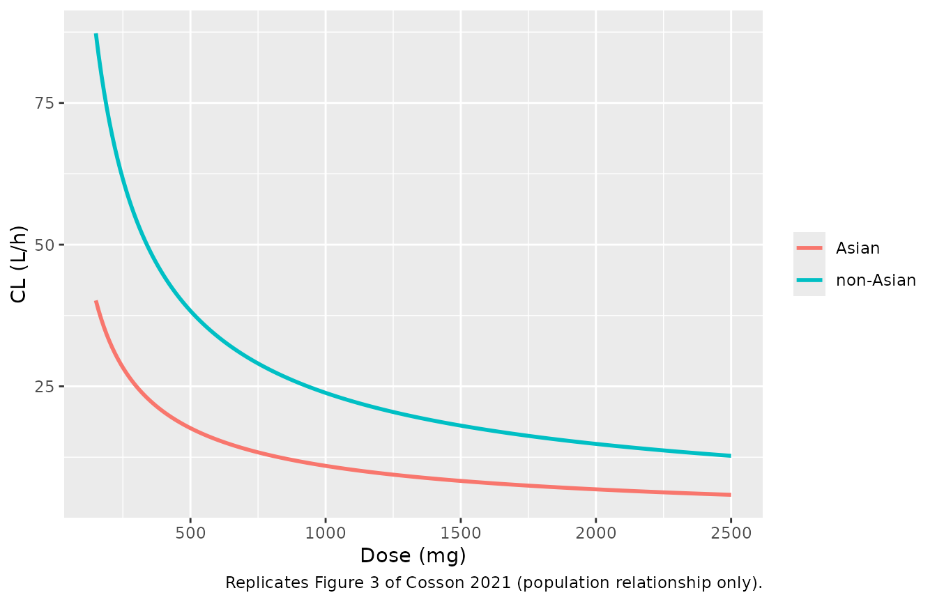
Replicates the population lines of Figure 3 of Cosson 2021: plasma clearance of linvencorvir versus dose in males.
Steady-state mass balance
Over one steady-state dosing interval the bioavailable dose must
equal what leaves the parent system: plasma clearance of
central plus conversion of liver to M5. Both
sides use the same typical parameters, so the difference is numerical
only (the authors’ Stirling approximation of log(N!) and the
1e-5 guards in the transit input contribute about
1e-4).
tau <- 24
ndose <- 27
t_ss <- (ndose - 1) * tau
obs_fine <- t_ss + seq(0, tau, by = 0.02)

make_typical <- function(dose, asian, sexf, fed = 0, id = 1L, times = obs_fine) {
  doses <- tibble(id = id, time = seq(0, t_ss, by = tau), evid = 1L,
                  amt = dose, cmt = "depot", dvid = NA_integer_)
  obs <- tibble(id = id, time = times, evid = 0L, amt = 0,
                cmt = "central", dvid = 1L)
  bind_rows(doses, obs) |>
    arrange(time, desc(evid)) |>
    mutate(DOSE_LINVENCORVIR_MG = dose, FED = fed, RACE_ASIAN = asian, SEXF = sexf)
}

trap <- function(t, y) sum(diff(t) * (head(y, -1) + tail(y, -1)) / 2)

mb <- as.data.frame(rxode2::rxSolve(
  mod_typ, make_typical(200, asian = 0, sexf = 0),
  returnType = "data.frame", atol = 1e-10, rtol = 1e-10
))
#> ℹ omega/sigma items treated as zero: 'etalvmax_uptake', 'etalkm_uptake', 'etalcl', 'etalvc', 'etalk_m5_form', 'etalcl_m5', 'etalka', 'etalmtt', 'etalntr', 'etalk_liver_central'
mb_ss <- mb[mb$time >= t_ss, ]
dose_in_mmol <- mod$theta[["e_fasted_fdepot"]] * 200 / 598.69
dose_out_mmol <- mb_ss$kel[1] * trap(mb_ss$time, mb_ss$central) +
  mb_ss$k_m5_form[1] * trap(mb_ss$time, mb_ss$liver)
mass_ratio <- dose_out_mmol / dose_in_mmol
mass_ratio
#> [1] 1.000148
stopifnot(abs(mass_ratio - 1) < 1e-3)
The transit input is driven by podo(depot) and
tad(depot) while f(depot) <- 0 keeps the
dose bolus itself out of the absorption compartment, exactly as the
control stream does with F1 = 0. The ratio above being 1
confirms that the input actually reaches the system.
Effect of sex and ethnicity at 600 mg q.d. (Figure 4)
grp <- expand.grid(asian = 0:1, sexf = 0:1)
fig4_ev <- bind_rows(lapply(seq_len(nrow(grp)), function(i) {
  make_typical(600, asian = grp$asian[i], sexf = grp$sexf[i], id = i,
               times = t_ss + seq(0, tau, by = 0.1))
}))
fig4 <- as.data.frame(rxode2::rxSolve(
  mod_typ, fig4_ev, keep = c("RACE_ASIAN", "SEXF"), returnType = "data.frame"
)) |>
  mutate(
    group = paste(ifelse(RACE_ASIAN == 1, "Asian", "non-Asian"),
                  ifelse(SEXF == 1, "female", "male")),
    tad = time - t_ss
  ) |>
  select(tad, group, `Linvencorvir plasma` = Cc, `M5 plasma` = Cc_m5) |>
  pivot_longer(-c(tad, group), names_to = "analyte", values_to = "conc")
#> ℹ omega/sigma items treated as zero: 'etalvmax_uptake', 'etalkm_uptake', 'etalcl', 'etalvc', 'etalk_m5_form', 'etalcl_m5', 'etalka', 'etalmtt', 'etalntr', 'etalk_liver_central'
#> Warning: multi-subject simulation without without 'omega'

ggplot(fig4, aes(tad, conc, colour = group)) +
  geom_line() +
  facet_wrap(~analyte, scales = "free_y") +
  scale_y_log10() +
  labs(x = "Time after dose at steady state (h)", y = "Concentration (ng/mL)",
       colour = NULL, caption = "Replicates Figure 4 of Cosson 2021.")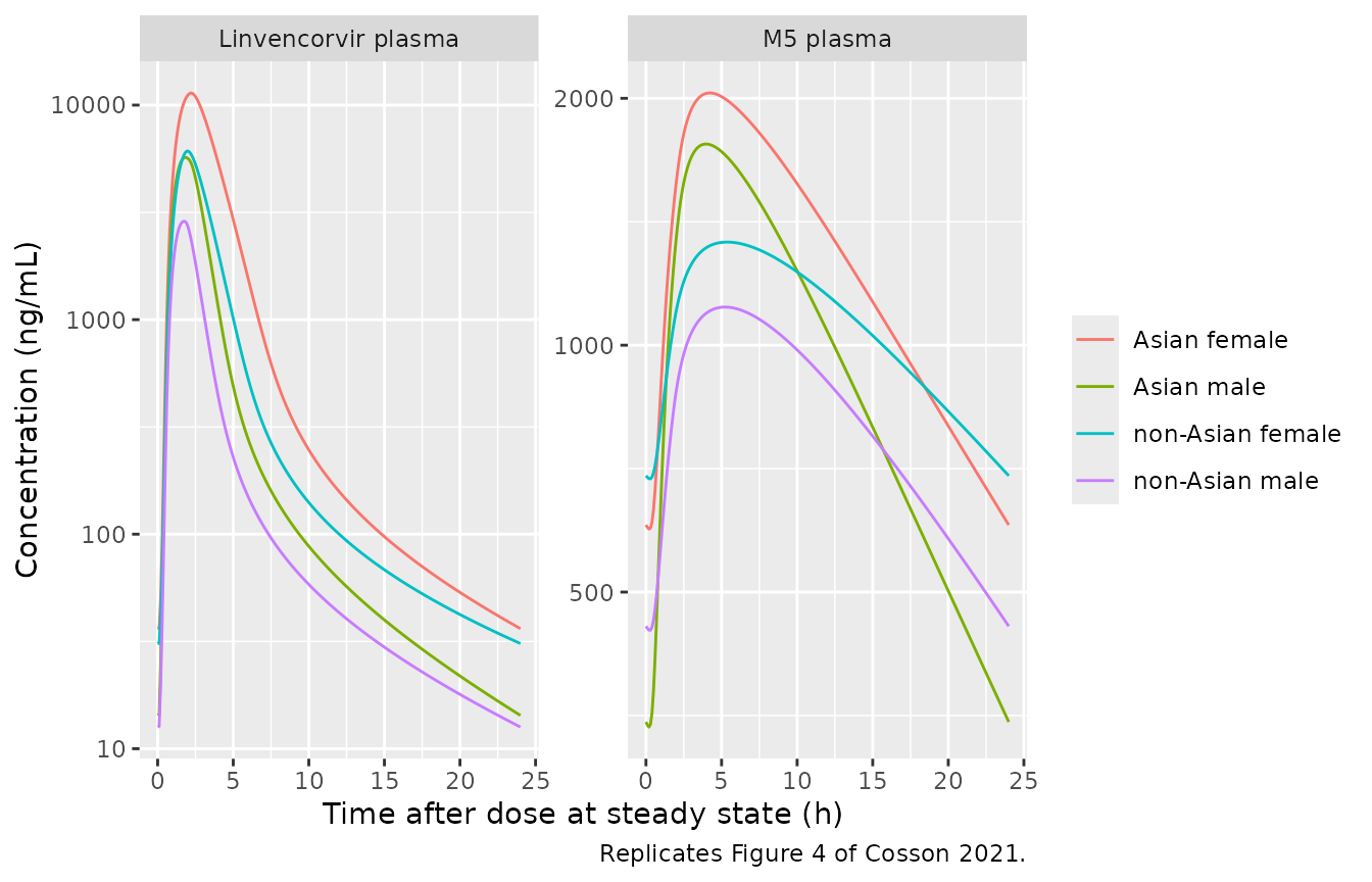
Replicates Figure 4 of Cosson 2021: typical steady-state profiles of linvencorvir and M5 after 600 mg q.d. fasted, by sex and ethnicity.
The typical exposure rises more than dose-proportionally, as reported: the nonlinear uptake and the dose-dependent clearance both act in that direction.
typ_auc <- sapply(c(200, 1000), function(d) {
  s <- as.data.frame(rxode2::rxSolve(mod_typ, make_typical(d, 0, 0), returnType = "data.frame"))
  s <- s[s$time >= t_ss, ]
  trap(s$time, s$Cc)
})
#> ℹ omega/sigma items treated as zero: 'etalvmax_uptake', 'etalkm_uptake', 'etalcl', 'etalvc', 'etalk_m5_form', 'etalcl_m5', 'etalka', 'etalmtt', 'etalntr', 'etalk_liver_central'
#> ℹ omega/sigma items treated as zero: 'etalvmax_uptake', 'etalkm_uptake', 'etalcl', 'etalvc', 'etalk_m5_form', 'etalcl_m5', 'etalka', 'etalmtt', 'etalntr', 'etalk_liver_central'
auc_ratio_1000_200 <- typ_auc[2] / typ_auc[1]
auc_ratio_1000_200
#> [1] 16.59251
stopifnot(auc_ratio_1000_200 > 5)
Virtual cohort
Cosson 2021 simulated 500 time courses in male and female Asian and non-Asian subjects at 200, 400, 600 and 1,000 mg q.d. fasted for 27 days (Table 2). The paper does not state how the two sexes were mixed. Equal numbers of males and females reproduce Table 2 closely, whereas males alone fall well below it, so the cohort below is sex-balanced: 100 males and 100 females per dose and ethnicity arm (200 per arm). Body weight and age do not enter the model.
set.seed(2021)
rxode2::rxSetSeed(2021)

n_per_sex <- 100L
obs_ss <- t_ss + c(0, seq(0.25, 4, by = 0.25), 5:24)

make_cohort <- function(dose, asian, sexf, n, id_offset) {
  ids <- id_offset + seq_len(n)
  doses <- expand.grid(id = ids, time = seq(0, t_ss, by = tau)) |>
    mutate(evid = 1L, amt = dose, cmt = "depot", dvid = NA_integer_)
  obs <- expand.grid(id = ids, time = obs_ss) |>
    mutate(evid = 0L, amt = 0, cmt = "central", dvid = 1L)
  bind_rows(doses, obs) |>
    mutate(
      DOSE_LINVENCORVIR_MG = dose, FED = 0, RACE_ASIAN = asian, SEXF = sexf,
      treatment = sprintf("%d mg %s", dose, ifelse(asian == 1, "Asian", "non-Asian"))
    )
}

arms <- expand.grid(dose = c(200L, 400L, 600L, 1000L), asian = 0:1, sexf = 0:1)
events <- bind_rows(lapply(seq_len(nrow(arms)), function(i) {
  make_cohort(arms$dose[i], arms$asian[i], arms$sexf[i],
              n = n_per_sex, id_offset = (i - 1L) * n_per_sex)
})) |>
  arrange(id, time, desc(evid)) |>
  relocate(id, time, evid, amt, cmt, dvid)

stopifnot(!anyDuplicated(events[, c("id", "time", "evid")]))
events |> distinct(id, treatment) |> count(treatment)
#>           treatment   n
#> 1     1000 mg Asian 200
#> 2 1000 mg non-Asian 200
#> 3      200 mg Asian 200
#> 4  200 mg non-Asian 200
#> 5      400 mg Asian 200
#> 6  400 mg non-Asian 200
#> 7      600 mg Asian 200
#> 8  600 mg non-Asian 200
Simulation
The model states are amounts in mmol (a 200 mg dose is 0.33 mmol), so
rxode2’s default absolute tolerance of 1e-8 mmol is coarse relative to
the trough amounts of high-clearance subjects and lets the solver return
slightly negative concentrations. The simulation therefore uses
atol = 1e-12. Any negative value that remains must be
numerical noise (checked below) and is set to zero before NCA.
sim <- as.data.frame(rxode2::rxSolve(
  mod, events,
  keep = c("treatment", "DOSE_LINVENCORVIR_MG", "RACE_ASIAN"),
  returnType = "data.frame", atol = 1e-12
)) |>
  mutate(liver_mg = 598.69 * liver)

# Fail loudly if a negative value is anything more than solver noise.
stopifnot(
  min(sim$Cc) > -1e-4,
  min(sim$Cc_m5) > -1e-4,
  min(sim$liver_mg) > -1e-6
)
sim <- sim |>
  mutate(
    Cc = pmax(Cc, 0),
    Cc_m5 = pmax(Cc_m5, 0),
    liver_mg = pmax(liver_mg, 0)
  )
Steady-state plasma and liver profiles at 600 mg q.d. (Figure 5)
fig5 <- sim |>
  filter(DOSE_LINVENCORVIR_MG == 600) |>
  mutate(
    Ethnicity = ifelse(RACE_ASIAN == 1, "Asian", "non-Asian"),
    tad = time - t_ss
  ) |>
  select(id, tad, Ethnicity,
         `Linvencorvir plasma (ng/mL)` = Cc,
         `Linvencorvir liver (mg)` = liver_mg,
         `M5 plasma (ng/mL)` = Cc_m5) |>
  pivot_longer(-c(id, tad, Ethnicity), names_to = "quantity", values_to = "value") |>
  group_by(tad, Ethnicity, quantity) |>
  summarise(
    q05 = quantile(value, 0.05), q50 = median(value), q95 = quantile(value, 0.95),
    .groups = "drop"
  )

ggplot(fig5, aes(tad, q50, colour = Ethnicity, fill = Ethnicity)) +
  geom_ribbon(aes(ymin = q05, ymax = q95), alpha = 0.2, colour = NA) +
  geom_line() +
  facet_wrap(~quantity, scales = "free_y") +
  scale_y_log10() +
  labs(x = "Time after dose at steady state (h)", y = NULL, colour = NULL, fill = NULL,
       caption = "Replicates Figure 5 of Cosson 2021.")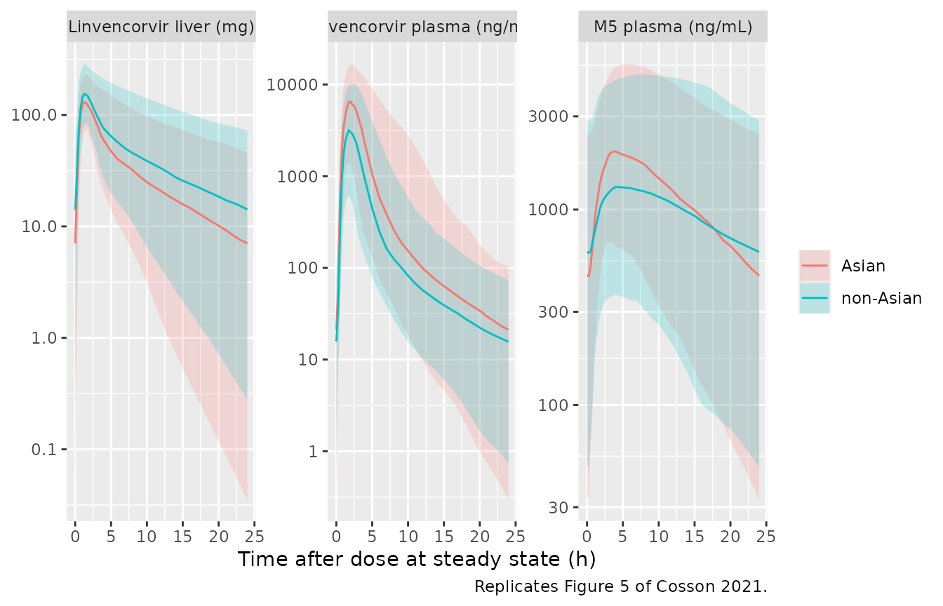
Replicates Figure 5 of Cosson 2021: median and 90% prediction interval of steady-state linvencorvir in plasma and liver and of M5 in plasma after 600 mg q.d. fasted, by ethnicity (200 simulated subjects per group; the paper used 1,000).
PKNCA validation
Table 2 reports steady-state Cmax and AUC over the 24 h dosing
interval for plasma linvencorvir and M5, and the maximum amount (Amax)
and area under the amount curve (AUQ) for linvencorvir in the liver, as
geometric means. The same PKNCA set-up is applied to each quantity; for
the liver, PKNCA’s cmax and auclast are Amax
and AUQ.
dose_df <- events |>
  filter(evid == 1) |>
  select(id, time, amt, treatment)
dose_obj <- PKNCA::PKNCAdose(dose_df, amt ~ time | treatment + id)

intervals <- data.frame(start = t_ss, end = t_ss + tau, cmax = TRUE, auclast = TRUE)

run_nca <- function(sim, column) {
  conc <- sim |>
    filter(!is.na(.data[[column]])) |>
    transmute(id, time, treatment, Cc = .data[[column]])
  # Time-zero anchor per subject (pre-dose amount is zero).
  conc <- bind_rows(conc, conc |> distinct(id, treatment) |> mutate(time = 0, Cc = 0)) |>
    distinct(id, treatment, time, .keep_all = TRUE) |>
    arrange(id, treatment, time)
  conc_obj <- PKNCA::PKNCAconc(conc, Cc ~ time | treatment + id)
  PKNCA::pk.nca(PKNCA::PKNCAdata(conc_obj, dose_obj, intervals = intervals))
}

nca_parent <- run_nca(sim, "Cc")
nca_liver <- run_nca(sim, "liver_mg")
nca_m5 <- run_nca(sim, "Cc_m5")

# Table 2 reports geometric means, so aggregate to geometric means here
# instead of the default median of ncaComparisonTable().
geo_mean <- function(nca) {
  as.data.frame(nca) |>
    filter(PPTESTCD %in% c("cmax", "auclast")) |>
    group_by(treatment, PPTESTCD) |>
    summarise(PPORRES = exp(mean(log(PPORRES))), .groups = "drop")
}
Comparison against published NCA
trt <- c(sprintf("%d mg non-Asian", c(200L, 400L, 600L, 1000L)),
         sprintf("%d mg Asian", c(200L, 400L, 600L, 1000L)))

# Cosson 2021 Table 2, geometric means (q.d. fasted, steady state).
pub_parent <- tibble(
  treatment = trt,
  cmax = c(396, 1607, 3614, 7706, 915, 3617, 6828, 15132),
  auclast = c(1353, 4654, 10732, 25200, 2794, 10429, 21334, 55089)
)
pub_liver <- tibble(
  treatment = trt,
  cmax = c(75.8, 125, 162, 230, 64.5, 106, 139, 208),
  auclast = c(530, 840, 1060, 1436, 385, 636, 803, 1180)
)
# M5 AUC is printed in mcg*h/mL; x 1000 gives ng*h/mL.
pub_m5 <- tibble(
  treatment = trt,
  cmax = c(633, 998, 1287, 1835, 935, 1530, 2011, 2990),
  auclast = 1000 * c(10.9, 17.3, 22.1, 30.5, 13.0, 21.7, 27.6, 40.2)
)

cmp_parent <- nlmixr2lib::ncaComparisonTable(
  geo_mean(nca_parent), pub_parent, by = "treatment",
  units = c(cmax = "ng/mL", auclast = "ng*h/mL")
)
cmp_liver <- nlmixr2lib::ncaComparisonTable(
  geo_mean(nca_liver), pub_liver, by = "treatment",
  units = c(cmax = "mg", auclast = "mg*h")
)
cmp_m5 <- nlmixr2lib::ncaComparisonTable(
  geo_mean(nca_m5), pub_m5, by = "treatment",
  units = c(cmax = "ng/mL", auclast = "ng*h/mL")
)

knitr::kable(cmp_parent, caption = "Plasma linvencorvir at steady state, simulated vs Table 2 geometric means. * differs by >20%.")| NCA parameter | treatment | Reference | Simulated | % diff |
|---|---|---|---|---|
| Cmax (ng/mL) | 200 mg non-Asian | 396 | 382 | -3.5% |
| Cmax (ng/mL) | 400 mg non-Asian | 1610 | 1760 | +9.4% |
| Cmax (ng/mL) | 600 mg non-Asian | 3610 | 3270 | -9.6% |
| Cmax (ng/mL) | 1000 mg non-Asian | 7710 | 7870 | +2.1% |
| Cmax (ng/mL) | 200 mg Asian | 915 | 931 | +1.8% |
| Cmax (ng/mL) | 400 mg Asian | 3620 | 3320 | -8.1% |
| Cmax (ng/mL) | 600 mg Asian | 6830 | 6530 | -4.3% |
| Cmax (ng/mL) | 1000 mg Asian | 15100 | 15600 | +3.1% |
| AUClast (ng*h/mL) | 200 mg non-Asian | 1350 | 1340 | -1.1% |
| AUClast (ng*h/mL) | 400 mg non-Asian | 4650 | 4980 | +7.0% |
| AUClast (ng*h/mL) | 600 mg non-Asian | 10700 | 9660 | -9.9% |
| AUClast (ng*h/mL) | 1000 mg non-Asian | 25200 | 25800 | +2.3% |
| AUClast (ng*h/mL) | 200 mg Asian | 2790 | 2770 | -0.9% |
| AUClast (ng*h/mL) | 400 mg Asian | 10400 | 9740 | -6.7% |
| AUClast (ng*h/mL) | 600 mg Asian | 21300 | 20600 | -3.5% |
| AUClast (ng*h/mL) | 1000 mg Asian | 55100 | 56700 | +3.0% |
knitr::kable(cmp_liver, caption = "Liver linvencorvir at steady state (Cmax row = Amax, AUClast row = AUQ), simulated vs Table 2 geometric means. * differs by >20%.")| NCA parameter | treatment | Reference | Simulated | % diff |
|---|---|---|---|---|
| Cmax (mg) | 200 mg non-Asian | 75.8 | 75.1 | -0.9% |
| Cmax (mg) | 400 mg non-Asian | 125 | 122 | -2.4% |
| Cmax (mg) | 600 mg non-Asian | 162 | 164 | +1.4% |
| Cmax (mg) | 1000 mg non-Asian | 230 | 223 | -2.9% |
| Cmax (mg) | 200 mg Asian | 64.5 | 65.1 | +0.9% |
| Cmax (mg) | 400 mg Asian | 106 | 107 | +0.6% |
| Cmax (mg) | 600 mg Asian | 139 | 139 | +0.2% |
| Cmax (mg) | 1000 mg Asian | 208 | 214 | +3.1% |
| AUClast (mg*h) | 200 mg non-Asian | 530 | 517 | -2.4% |
| AUClast (mg*h) | 400 mg non-Asian | 840 | 805 | -4.2% |
| AUClast (mg*h) | 600 mg non-Asian | 1060 | 1090 | +2.7% |
| AUClast (mg*h) | 1000 mg non-Asian | 1440 | 1360 | -5.5% |
| AUClast (mg*h) | 200 mg Asian | 385 | 384 | -0.4% |
| AUClast (mg*h) | 400 mg Asian | 636 | 636 | +0.0% |
| AUClast (mg*h) | 600 mg Asian | 803 | 802 | -0.1% |
| AUClast (mg*h) | 1000 mg Asian | 1180 | 1210 | +2.5% |
knitr::kable(cmp_m5, caption = "Plasma M5 at steady state, simulated vs Table 2 geometric means. * differs by >20%.")| NCA parameter | treatment | Reference | Simulated | % diff |
|---|---|---|---|---|
| Cmax (ng/mL) | 200 mg non-Asian | 633 | 603 | -4.8% |
| Cmax (ng/mL) | 400 mg non-Asian | 998 | 971 | -2.7% |
| Cmax (ng/mL) | 600 mg non-Asian | 1290 | 1340 | +4.3% |
| Cmax (ng/mL) | 1000 mg non-Asian | 1840 | 1690 | -8.0% |
| Cmax (ng/mL) | 200 mg Asian | 935 | 920 | -1.6% |
| Cmax (ng/mL) | 400 mg Asian | 1530 | 1630 | +6.6% |
| Cmax (ng/mL) | 600 mg Asian | 2010 | 1970 | -1.9% |
| Cmax (ng/mL) | 1000 mg Asian | 2990 | 3120 | +4.4% |
| AUClast (ng*h/mL) | 200 mg non-Asian | 10900 | 10300 | -5.4% |
| AUClast (ng*h/mL) | 400 mg non-Asian | 17300 | 16900 | -2.1% |
| AUClast (ng*h/mL) | 600 mg non-Asian | 22100 | 23100 | +4.3% |
| AUClast (ng*h/mL) | 1000 mg non-Asian | 30500 | 28300 | -7.1% |
| AUClast (ng*h/mL) | 200 mg Asian | 13000 | 12800 | -1.8% |
| AUClast (ng*h/mL) | 400 mg Asian | 21700 | 22800 | +5.0% |
| AUClast (ng*h/mL) | 600 mg Asian | 27600 | 27400 | -0.9% |
| AUClast (ng*h/mL) | 1000 mg Asian | 40200 | 42100 | +4.8% |
# ncaComparisonTable() returns character columns such as "+9.4%" or "-21.0%*".
pct_diff <- function(cmp) {
  as.numeric(gsub("[%*]", "", cmp[["% diff"]]))
}
all_pct <- c(pct_diff(cmp_parent), pct_diff(cmp_liver), pct_diff(cmp_m5))
summary(all_pct)
#>    Min. 1st Qu.  Median    Mean 3rd Qu.    Max.
#> -9.9000 -3.5000 -0.9000 -0.6917  2.5500  9.4000
# Centre and robust envelope over all 48 cells: a mis-transcribed parameter
# or unit moves the whole set.
stopifnot(
  length(all_pct) == 48L,
  !anyNA(all_pct),
  abs(median(all_pct)) < 10,
  quantile(abs(all_pct), 0.9) < 25
)
Asian versus non-Asian: plasma versus liver
The paper’s central conclusion is that plasma linvencorvir exposure is about twice as high in Asians while the liver exposure is similar or lower (Table 2 geometric mean ratios 1.99-2.24 for plasma AUC and 0.73-0.82 for liver AUQ).
gmr <- bind_rows(
  geo_mean(nca_parent) |> mutate(quantity = "Plasma linvencorvir"),
  geo_mean(nca_liver) |> mutate(quantity = "Liver linvencorvir"),
  geo_mean(nca_m5) |> mutate(quantity = "Plasma M5")
) |>
  filter(PPTESTCD == "auclast") |>
  separate(treatment, into = c("dose", "unit", "ethnicity"), sep = " ") |>
  select(quantity, dose, ethnicity, PPORRES) |>
  pivot_wider(names_from = ethnicity, values_from = PPORRES) |>
  mutate(simulated = Asian / `non-Asian`, dose = as.integer(dose)) |>
  arrange(quantity, dose)

gmr_pub <- tibble(
  quantity = rep(c("Liver linvencorvir", "Plasma M5", "Plasma linvencorvir"), each = 4),
  dose = rep(c(200L, 400L, 600L, 1000L), 3),
  published = c(0.73, 0.76, 0.76, 0.82, 1.19, 1.25, 1.25, 1.32, 2.07, 2.24, 1.99, 2.19)
)
gmr_tab <- gmr |>
  left_join(gmr_pub, by = c("quantity", "dose")) |>
  transmute(quantity, dose, simulated = signif(simulated, 3), published)
gmr_tab |>
  rename(`Quantity (AUC or AUQ)` = quantity, `Dose (mg)` = dose,
         `Simulated GMR` = simulated, `Table 2 GMR` = published) |>
knitr::kable(caption = "Geometric mean ratio Asian / non-Asian of steady-state AUC (plasma) or AUQ (liver).")| Quantity (AUC or AUQ) | Dose (mg) | Simulated GMR | Table 2 GMR |
|---|---|---|---|
| Liver linvencorvir | 200 | 0.741 | 0.73 |
| Liver linvencorvir | 400 | 0.791 | 0.76 |
| Liver linvencorvir | 600 | 0.736 | 0.76 |
| Liver linvencorvir | 1000 | 0.891 | 0.82 |
| Plasma M5 | 200 | 1.240 | 1.19 |
| Plasma M5 | 400 | 1.350 | 1.25 |
| Plasma M5 | 600 | 1.190 | 1.25 |
| Plasma M5 | 1000 | 1.490 | 1.32 |
| Plasma linvencorvir | 200 | 2.070 | 2.07 |
| Plasma linvencorvir | 400 | 1.960 | 2.24 |
| Plasma linvencorvir | 600 | 2.130 | 1.99 |
| Plasma linvencorvir | 1000 | 2.200 | 2.19 |
med_gmr <- gmr_tab |> group_by(quantity) |> summarise(m = median(simulated))
med_gmr
#> # A tibble: 3 × 2
#>   quantity                m
#>   <chr>               <dbl>
#> 1 Liver linvencorvir  0.766
#> 2 Plasma M5           1.30
#> 3 Plasma linvencorvir 2.1
stopifnot(
  med_gmr$m[med_gmr$quantity == "Plasma linvencorvir"] > 1.5,
  med_gmr$m[med_gmr$quantity == "Liver linvencorvir"] < 1
)
Assumptions and deviations
- Residual-error correlation not carried. The published model correlates the two proportional errors (covariance 0.0418, correlation 0.404) and the two additive errors (covariance 34.8, correlation 0.843) across linvencorvir and M5. nlmixr2 cannot express a residual correlation between endpoints, so each endpoint keeps its marginal combined additive + proportional error. This affects only simulated observations with residual noise, not individual predictions.
-
Dose covariate. Plasma clearance depends on the
nominal treatment-arm dose (
TRTin the control stream), carried here asDOSE_LINVENCORVIR_MG. It is read as the dose per administration, consistent with the paper’s reference “CL when dose equals 200 mg” and with Figure 3, whose dose axis spans the single-dose range to 2,500 mg. The value must be supplied by the user and is not derived from the dose records. - Transit input uses the most recent dose only. As in the control stream, the Savic transit input is computed from the last dose amount and the time since that dose; input from an earlier dose that is still in transit is dropped when the next dose is given. With a mean transit time of 0.36-1.17 h and dosing every 12 or 24 h this is immaterial.
-
Log-factorial approximation kept. The transit input
uses the Stirling approximation of log(N!) and the
1e-5numerical guards written in the control stream rather than the exactlgamma(N + 1), to match the fitted model. - Units of the Michaelis-Menten constants. Table 1 gives Vm in mmol/h and Km in mmol, and the control stream applies them to compartment amounts in mmol; they are used exactly that way here, so the uptake saturates on the amount in the absorption or plasma compartment rather than on a concentration.
-
Liver amount units. The control stream’s liver
output
LRO = 1000 * MWRO * A(2)is in micrograms, while the corrected Table 2 (correction dated 24 March 2021) reports Amax and AUQ in mg. The simulated liver amounts in mg (598.69 * liver) reproduce the Table 2 values, which confirms the corrected units. - Sex mix of the Table 2 cohort. The paper simulated male and female subjects but does not give their proportion; the maintainers used equal numbers because that reproduces Table 2, whereas an all-male cohort underpredicts it.
- Cohort size. 200 subjects per dose and ethnicity arm instead of the paper’s 500 per group, following this package’s cap on simulated cohort size.
-
K32 has no between-subject variability. The control
stream carries an
ETA(11)on K32 fixed to 0, so no eta is declared for it. - No separate erratum or correction notice beyond the in-article correction of the Table 2 liver units was found as of 2026-09-28.