Caspofungin (Yang 2022)
Source:vignettes/articles/Yang_2022_caspofungin.Rmd
Yang_2022_caspofungin.RmdModel and source
- Citation: Yang Q, Zhang T, Zhang Y, Sun D, Zheng X, Du Q, Wang X, Cheng X, Xing J, Dong Y. The recommended dosage regimen for caspofungin in patients with higher body weight or hypoalbuminaemia will result in low exposure: five years of data based on a population pharmacokinetic model and Monte-Carlo simulations. Front Pharmacol. 2022;13:993330. doi:10.3389/fphar.2022.993330. PMCID: PMC9669616.
- Article: https://doi.org/10.3389/fphar.2022.993330
- Open-access full text: https://www.ncbi.nlm.nih.gov/pmc/articles/PMC9669616/
Yang 2022 fitted two separate one-compartment population PK models to caspofungin concentrations, and both are in nlmixr2lib:
-
Yang_2022_caspofungin: One-compartment population PK model for intravenous caspofungin in hospitalised Chinese adults with confirmed or probable candidiasis (ICU, solid-organ transplant, haematology and respiratory patients; the ‘general PPK model’ of Yang 2022). Clearance and volume each carry two dichotomised covariates, hypoalbuminaemia (serum albumin < 35 g/L) and body weight >= 70 kg, entering as (1 + theta x indicator) factors. Log-normal IIV on CL and V and a proportional residual error. A separately fitted ICU-subgroup model from the same paper is Yang_2022_caspofungin_icu. -
Yang_2022_caspofungin_icu: One-compartment population PK model for intravenous caspofungin in critically ill adults in the intensive care unit (the ‘ICU-subgroup PPK model’ of Yang 2022), pooling 51 ICU patients from Xi’an, China with 85 ICU patients digitised from seven published caspofungin studies. Clearance carries one dichotomised covariate, body weight >= 70 kg, entering as a (1 + theta x indicator) factor; volume has no covariate. Log-normal IIV on CL and V and a proportional residual error. The general-population model from the same paper is Yang_2022_caspofungin.
Both models enter albumin and weight as yes/no indicators, never as continuous values. The general model has
CL = 0.32 x (1 + 0.46 ALB*) x (1 + 0.98 WT*) x exp(eta_CL), V = 13.31 x (1 + 0.49 ALB*) x (1 + 0.24 WT*) x exp(eta_V),
with ALB* = 1 for albumin < 35 g/L and WT* = 1 for weight >= 70 kg. The ICU model has CL = 0.42 x (1 + 0.34 WT*) x exp(eta_CL) and V = 10.20 x exp(eta_V).
The paper then simulates the steady-state AUC over 24 h as AUC24 = Dose / CL and computes the probability of reaching the free AUC24/MIC targets of 20 (C. albicans) and 7 (C. parapsilosis, C. glabrata), with 97% protein binding.
Read the weight coefficients with care. As printed in Table 3, a weight of 70 kg or more nearly doubles clearance (x 1.98) and raises volume by 24%. The paper’s own simulations (Figure 5A, Table S1) and its mean individual clearances (Table 4) all fit the opposite assignment, x 1.24 on clearance. The model file carries the printed values. The section Weight coefficients below runs both readings against those outputs.
Population
The general model used 921 plasma concentrations from 299 adults with confirmed or probable candidiasis treated at the First Affiliated Hospital of Xi’an Jiaotong University between June 2014 and June 2019 (Methods 2.1-2.3, Table 1). There were 51 ICU, 163 solid-organ transplant, 42 haematology and 43 other patients. Mean age was 44 years (18-99), mean weight 62.3 kg (30-100), 92 were women, and mean albumin was 35.6 g/L (15.1-64.5), with 161 below 35 g/L. Caspofungin was given as a 1 h intravenous infusion, mostly 70 mg on day 1 and then 50 mg daily, with 70/35 mg in Child-Pugh B hepatic impairment and 70/70 mg above 75 kg. Most samples were sparse therapeutic drug monitoring samples (median three per patient).
The ICU model pooled the hospital’s 51 ICU patients with 85 ICU patients whose concentrations the authors took from seven published studies (Supplementary 3.1.2). The 136 patients had a mean age of 60.5 years and a mean weight of 68.1 kg; the literature patients were heavier (78.7 kg) than the hospital’s (60.7 kg). Mean albumin was 28.0 g/L, and 50 were on continuous renal replacement therapy.
Source trace
No control stream was published. The supplement holds text and the PTA Tables S1 and S2 only.
| Model element | Value | Source location |
|---|---|---|
| One-compartment model, 1 h IV infusion | – | Methods 2.1 (‘intravenously over 1 h’); Results 3.2.1 |
| General: CL and V equations, ALB* and WT* definitions | – | Table 3, footnote c |
General lcl (theta1) |
0.32 L/h | Table 3, final model |
General lvc (theta2) |
13.31 L | Table 3 |
General e_alb_cl (theta3) |
0.46 | Table 3 |
General e_alb_vc (theta4) |
0.49 | Table 3 |
General e_wt_cl (theta5) |
0.98 | Table 3 (see Weight coefficients) |
General e_wt_vc (theta6) |
0.24 | Table 3 |
General etalcl, etalvc
|
29.2%, 59.2% | Table 3, ‘Inter-individual variability (%)’ |
General propSd
|
0.193 | Table 3, ‘Proportional (%)’ 19.3 |
| ICU: CL and V equations | – | Table 3, footnote d |
ICU lcl (theta1) |
0.42 L/h | Table 3, final model |
ICU lvc (theta2) |
10.20 L | Table 3 |
ICU e_wt_cl (theta3) |
0.34 | Table 3 |
ICU etalcl, etalvc
|
13.5%, 19.6% | Table 3 |
ICU propSd
|
0.243 | Table 3, ‘Proportional (%)’ 24.3 |
| AUC24 = Dose / CL; fAUC24/MIC targets; 97% binding | – | Methods 2.6 |
Typical values
The covariate equations are checked against hand calculation, for both models, in every albumin and weight category.
mod_gen <- readModelDb("Yang_2022_caspofungin")
mod_icu <- readModelDb("Yang_2022_caspofungin_icu")

# One observation per covariate combination; zeroRe() gives the typical values.
typical_values <- function(model, cov) {
  ev <- cov
  ev$id <- seq_len(nrow(ev))
  ev$time <- 0
  ev$evid <- 0
  ev$amt <- 0
  ev$cmt <- "central"
  # zeroRe() removes every eta, so rxSolve()'s 'without omega' warning is expected.
  out <- suppressWarnings(rxode2::rxSolve(rxode2::zeroRe(model), ev, returnType = "data.frame"))
  cbind(cov, cl = out$cl, vc = out$vc)
}

combos <- expand.grid(ALB = c(30, 40), WT = c(60, 80))
typ_gen <- typical_values(mod_gen, combos)
#> ℹ parameter labels from comments will be replaced by 'label()'
#> ℹ omega/sigma items treated as zero: 'etalcl', 'etalvc'
typ_icu <- typical_values(mod_icu, combos)
#> ℹ parameter labels from comments will be replaced by 'label()'
#> ℹ omega/sigma items treated as zero: 'etalcl', 'etalvc'

hand_cl <- with(combos, 0.32 * (1 + 0.46 * (ALB < 35)) * (1 + 0.98 * (WT >= 70)))
hand_vc <- with(combos, 13.31 * (1 + 0.49 * (ALB < 35)) * (1 + 0.24 * (WT >= 70)))
stopifnot(
  all(abs(typ_gen$cl - hand_cl) < 1e-10),
  all(abs(typ_gen$vc - hand_vc) < 1e-10),
  all(abs(typ_icu$cl - 0.42 * (1 + 0.34 * (combos$WT >= 70))) < 1e-10),
  all(abs(typ_icu$vc - 10.20) < 1e-10)
)

# The 70 kg threshold is inclusive (WT* = 1 at weight >= 70 kg).
edge <- typical_values(mod_gen, data.frame(ALB = 40, WT = c(69.9, 70)))
#> ℹ parameter labels from comments will be replaced by 'label()'
#> ℹ omega/sigma items treated as zero: 'etalcl', 'etalvc'
stopifnot(abs(edge$cl[2] / edge$cl[1] - 1.98) < 1e-10)

dplyr::bind_rows(
  dplyr::mutate(typ_gen, model = "General"),
  dplyr::mutate(typ_icu, model = "ICU subgroup")
) |>
  dplyr::mutate(
    ALB = ifelse(ALB < 35, "< 35 g/L", ">= 35 g/L"),
    WT = ifelse(WT >= 70, ">= 70 kg", "< 70 kg")
  ) |>
  dplyr::select(model, ALB, WT, cl, vc) |>
  dplyr::rename("Model" = model, "Albumin" = ALB, "Weight" = WT, "CL (L/h)" = cl, "V (L)" = vc) |>
knitr::kable(digits = 3, caption = "Typical clearance and volume by covariate category (Table 3).")| Model | Albumin | Weight | CL (L/h) | V (L) |
|---|---|---|---|---|
| General | < 35 g/L | < 70 kg | 0.467 | 19.832 |
| General | >= 35 g/L | < 70 kg | 0.320 | 13.310 |
| General | < 35 g/L | >= 70 kg | 0.925 | 24.592 |
| General | >= 35 g/L | >= 70 kg | 0.634 | 16.504 |
| ICU subgroup | < 35 g/L | < 70 kg | 0.420 | 10.200 |
| ICU subgroup | >= 35 g/L | < 70 kg | 0.420 | 10.200 |
| ICU subgroup | < 35 g/L | >= 70 kg | 0.563 | 10.200 |
| ICU subgroup | >= 35 g/L | >= 70 kg | 0.563 | 10.200 |
Virtual cohorts
Three cohorts of 200 subjects mirror the three groups of Table 4:
- all hospital patients, simulated with the general model: weight from Table 1 (62.3 +/- 11.5 kg, 30-100) and 161 of 299 hypoalbuminaemic;
- the hospital’s ICU patients, simulated with the general model: weight 60.7 +/- 11.5 kg (30-86) and 44 of 51 hypoalbuminaemic (Supplementary 3.4.1);
- the ICU subgroup, simulated with the ICU model: 51 of 136 drawn like the hospital’s ICU patients and 85 of 136 like the literature patients (78.7 +/- 6.1 kg, 48-139).
Only the albumin and weight categories enter the models, so albumin is drawn uniformly within its category. Weights outside a cohort’s range are redrawn, not clipped.
set.seed(2022)
rxode2::rxSetSeed(2022)
n_arm <- 200

draw_wt <- function(n, mu, sd, lo, hi) {
  out <- numeric(0)
  while (length(out) < n) {
    x <- rnorm(n, mu, sd)
    out <- c(out, x[x >= lo & x <= hi])
  }
  out[seq_len(n)]
}
draw_alb <- function(n, p_low) {
  low <- runif(n) < p_low
  ifelse(low, runif(n, 15.1, 35 - 1e-6), runif(n, 35, 64.5))
}

n_icu_hosp <- round(n_arm * 51 / 136)
subj <- dplyr::bind_rows(
  data.frame(
    group = "All patients (general model)",
    WT = draw_wt(n_arm, 62.3, 11.5, 30, 100), ALB = draw_alb(n_arm, 161 / 299)
  ),
  data.frame(
    group = "ICU patients (general model)",
    WT = draw_wt(n_arm, 60.7, 11.5, 30, 86), ALB = draw_alb(n_arm, 44 / 51)
  ),
  data.frame(
    group = "ICU subgroup (ICU model)",
    WT = c(
      draw_wt(n_icu_hosp, 60.7, 11.5, 30, 86),
      draw_wt(n_arm - n_icu_hosp, 78.7, 6.1, 48, 139)
    ),
    ALB = draw_alb(n_arm, 1)
  )
)
subj$id <- seq_len(nrow(subj))

subj |>
  dplyr::group_by(group) |>
  dplyr::summarise(
    mean_wt = mean(WT), pct_wt70 = 100 * mean(WT >= 70),
    pct_alb35 = 100 * mean(ALB < 35), .groups = "drop"
  ) |>
  dplyr::rename(
    "Cohort" = group, "Mean weight (kg)" = mean_wt,
    "Weight >= 70 kg (%)" = pct_wt70, "Albumin < 35 g/L (%)" = pct_alb35
  ) |>
knitr::kable(digits = 1, caption = "Virtual cohorts.")| Cohort | Mean weight (kg) | Weight >= 70 kg (%) | Albumin < 35 g/L (%) |
|---|---|---|---|
| All patients (general model) | 62.1 | 27.5 | 55 |
| ICU patients (general model) | 60.7 | 22.5 | 87 |
| ICU subgroup (ICU model) | 72.4 | 67.0 | 100 |
Each subject receives 70 mg on day 1 and then 50 mg daily for 28 days, each as a 1 h infusion. With a volume IIV of 59%, the slowest subjects have half-lives of several days, so steady state is assessed on day 28.
inf_dur <- 1
n_dose <- 28
tau <- 24
t_last <- (n_dose - 1) * tau
obs_times <- sort(unique(c(
  seq(0, 48, by = 0.5),
  seq(0, n_dose * tau, by = tau),
  t_last + seq(0, tau, by = 0.25)
)))

events <- dplyr::bind_rows(lapply(seq_len(nrow(subj)), function(i) {
  s <- subj[i, ]
  dose <- data.frame(
    id = s$id, time = (seq_len(n_dose) - 1) * tau, evid = 1,
    amt = c(70, rep(50, n_dose - 1)), cmt = "central"
  )
  dose$rate <- dose$amt / inf_dur
  obs <- data.frame(id = s$id, time = obs_times, evid = 0, amt = 0, rate = 0, cmt = "central")
  ev <- rbind(dose, obs)
  ev$WT <- s$WT
  ev$ALB <- s$ALB
  ev$group <- s$group
  ev[order(ev$time, -ev$evid), ]
}))
Simulation
sim <- dplyr::bind_rows(
  rxode2::rxSolve(
    mod_gen, dplyr::filter(events, group != "ICU subgroup (ICU model)"),
    keep = "group", returnType = "data.frame"
  ),
  rxode2::rxSolve(
    mod_icu, dplyr::filter(events, group == "ICU subgroup (ICU model)"),
    keep = "group", returnType = "data.frame"
  )
)
#> ℹ parameter labels from comments will be replaced by 'label()'
#> ℹ parameter labels from comments will be replaced by 'label()'
sim |>
  dplyr::filter(time <= 48) |>
  dplyr::group_by(group, time) |>
  dplyr::summarise(
    med = median(Cc), lo = quantile(Cc, 0.05), hi = quantile(Cc, 0.95),
    .groups = "drop"
  ) |>
  ggplot(aes(time, med, colour = group, fill = group)) +
  geom_ribbon(aes(ymin = lo, ymax = hi), alpha = 0.15, colour = NA) +
  geom_line() +
  labs(
    x = "Time after first dose (h)", y = "Caspofungin (mg/L)", colour = NULL, fill = NULL,
    caption = "Simulated median and 5th-95th percentiles; 70 mg then 50 mg daily, 1 h infusion."
  ) +
  theme_bw() +
  theme(legend.position = "bottom", legend.direction = "vertical")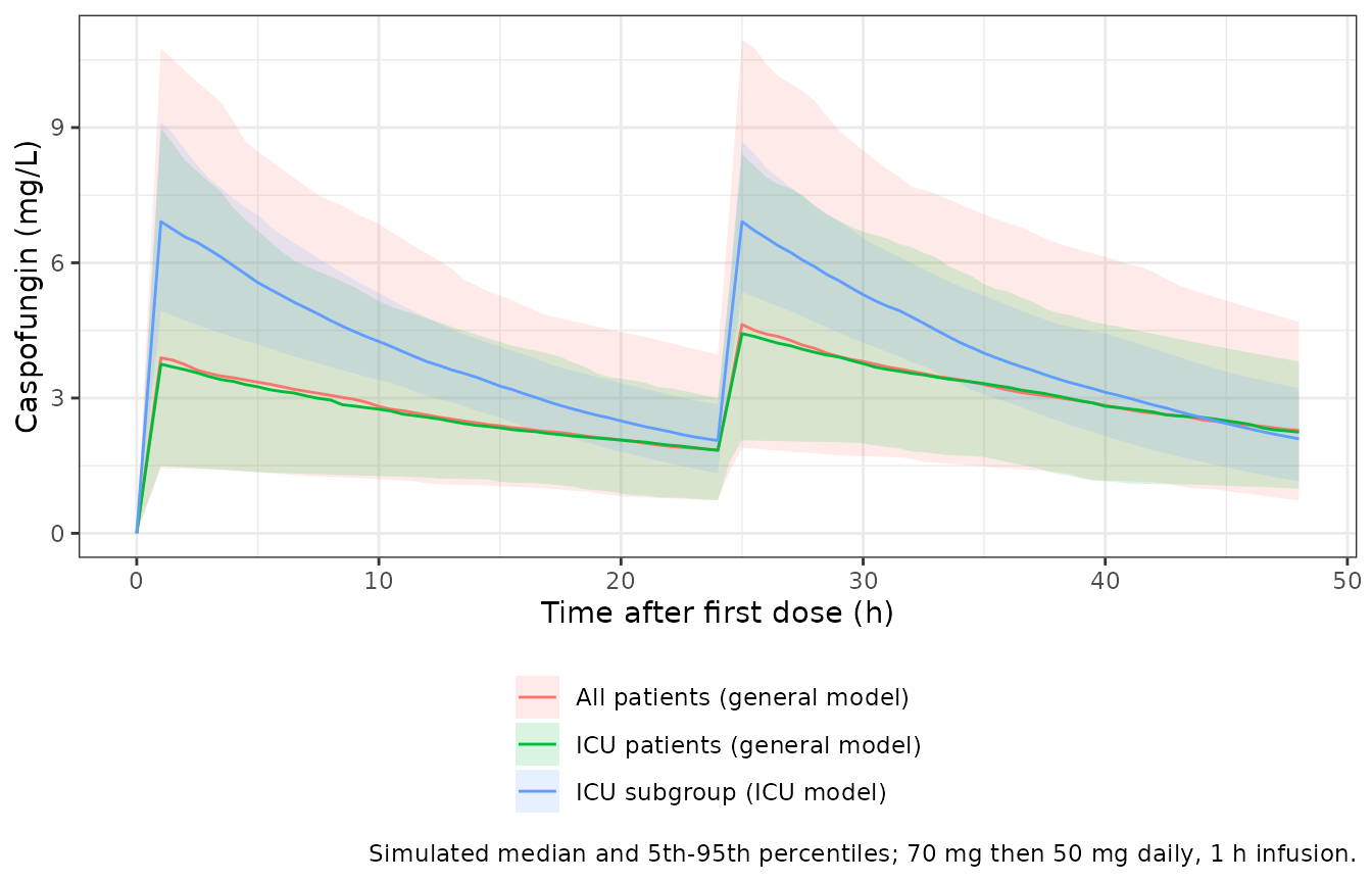
PKNCA validation
conc <- sim |>
  dplyr::filter(!is.na(Cc)) |>
  dplyr::select(id, time, Cc, group)
dose <- events |>
  dplyr::filter(evid == 1) |>
  dplyr::select(id, time, amt, group)
conc_obj <- PKNCA::PKNCAconc(conc, Cc ~ time | group + id, concu = "mg/L", timeu = "h")
dose_obj <- PKNCA::PKNCAdose(dose, amt ~ time | group + id, doseu = "mg")
intervals <- data.frame(
  start = t_last, end = t_last + tau, cmax = TRUE, cmin = TRUE, auclast = TRUE
)
nca_res <- as.data.frame(PKNCA::pk.nca(PKNCA::PKNCAdata(conc_obj, dose_obj, intervals = intervals))$result)

nca_res |>
  dplyr::filter(PPTESTCD %in% c("cmax", "cmin", "auclast")) |>
  dplyr::group_by(group, PPTESTCD) |>
  dplyr::summarise(
    mean = mean(PPORRES), median = median(PPORRES),
    q05 = quantile(PPORRES, 0.05), q95 = quantile(PPORRES, 0.95), .groups = "drop"
  ) |>
  dplyr::mutate(parameter = nlmixr2lib::ncaParamLabel(PPTESTCD)) |>
  dplyr::select(group, parameter, mean, median, q05, q95) |>
  dplyr::rename(
    "Cohort" = group, "NCA parameter" = parameter, "Mean" = mean, "Median" = median,
    "5th percentile" = q05, "95th percentile" = q95
  ) |>
knitr::kable(digits = 2, caption = "Simulated steady-state NCA, day 28 (Cmax, Cmin in mg/L; AUC in mg.h/L).")| Cohort | NCA parameter | Mean | Median | 5th percentile | 95th percentile |
|---|---|---|---|---|---|
| All patients (general model) | AUClast | 112.23 | 108.97 | 44.53 | 197.20 |
| All patients (general model) | Cmax | 6.57 | 6.06 | 2.62 | 11.85 |
| All patients (general model) | Cmin | 3.30 | 3.08 | 0.84 | 6.44 |
| ICU patients (general model) | AUClast | 103.34 | 100.61 | 46.84 | 175.34 |
| ICU patients (general model) | Cmax | 6.03 | 5.84 | 3.10 | 10.04 |
| ICU patients (general model) | Cmin | 3.05 | 2.84 | 1.01 | 6.00 |
| ICU subgroup (ICU model) | AUClast | 99.76 | 95.71 | 74.04 | 135.20 |
| ICU subgroup (ICU model) | Cmax | 7.06 | 7.09 | 5.62 | 8.62 |
| ICU subgroup (ICU model) | Cmin | 2.20 | 2.10 | 1.12 | 3.46 |
The paper’s AUC24 = Dose / CL is the steady-state AUC over one dosing interval. The model’s individual clearances are checked against it on day 28.
ind_cl <- sim |>
  dplyr::group_by(id) |>
  dplyr::summarise(cl = cl[1], .groups = "drop")
auc_ss <- nca_res |>
  dplyr::filter(PPTESTCD == "auclast") |>
  dplyr::left_join(ind_cl, by = "id") |>
  dplyr::mutate(ratio = PPORRES * cl / 50)
summary(auc_ss$ratio)
#>    Min. 1st Qu.  Median    Mean 3rd Qu.    Max.
#>  0.9578  1.0000  1.0000  0.9998  1.0000  1.0000
# The individual clearance is the one used in the solve; a ratio below 1 can
# only come from a slow subject not yet at steady state on day 28.
stopifnot(
  abs(median(auc_ss$ratio) - 1) < 0.005,
  quantile(abs(auc_ss$ratio - 1), 0.9) < 0.02
)
Comparison against Table 4
Table 4 gives the mean and SD of the individual (post hoc) AUC and CL in each group. The patients’ AUCs used their actual maintenance doses, mostly 50 mg.
published <- data.frame(
  group = c("All patients (general model)", "ICU patients (general model)", "ICU subgroup (ICU model)"),
  auclast = c(126.46, 101.46, 101.83)
)
sim_mean <- nca_res |>
  dplyr::filter(PPTESTCD == "auclast") |>
  dplyr::group_by(group) |>
  dplyr::summarise(auclast = mean(PPORRES), .groups = "drop")
cmp <- nlmixr2lib::ncaComparisonTable(
  simulated = sim_mean,
  reference = published,
  by = "group",
  params = "auclast",
  units = c(auclast = "mg*h/L"),
  tolerance_pct = 20
)
knitr::kable(cmp, caption = "Simulated vs published mean steady-state AUC24 (Table 4). * differs by >20%.")| NCA parameter | group | Reference | Simulated | % diff |
|---|---|---|---|---|
| AUClast (mg*h/L) | All patients (general model) | 126 | 112 | -11.3% |
| AUClast (mg*h/L) | ICU patients (general model) | 101 | 103 | +1.9% |
| AUClast (mg*h/L) | ICU subgroup (ICU model) | 102 | 99.8 | -2.0% |
# Centre of the distribution (one value per subject): a mis-transcribed
# clearance or covariate moves the mean by far more than this.
cmp_chk <- dplyr::left_join(sim_mean, published, by = "group", suffix = c("_sim", "_pub"))
stopifnot(all(abs(cmp_chk$auclast_sim / cmp_chk$auclast_pub - 1) < 0.25))
The ICU model and the general model’s ICU group match Table 4. For all patients the general model, as printed, gives a mean AUC about 11% below Table 4; the next section compares this with the alternative reading of the weight coefficient.
Weight coefficients
Table 3 gives theta5 (weight on CL) = 0.98 and theta6 (weight on V) =
0.24, and the bootstrap means (1.02 and 0.23) agree. Three outputs in
the same paper instead fit 0.24 on clearance, as if theta5 and theta6
were swapped. The volume coefficient cannot be checked, because AUC24 =
Dose / CL does not depend on V. Below, “printed” is the model as shipped
and “swapped” is the same model with e_wt_cl = 0.24 and
e_wt_vc = 0.98.
mod_swap <- rxode2::rxode2(mod_gen) |> rxode2::ini(e_wt_cl = 0.24, e_wt_vc = 0.98)
#> ℹ parameter labels from comments will be replaced by 'label()'
#> ℹ change initial estimate of `e_wt_cl` to `0.24`
#> ℹ change initial estimate of `e_wt_vc` to `0.98`
typ_swap <- typical_values(mod_swap, combos)
#> ℹ omega/sigma items treated as zero: 'etalcl', 'etalvc'
omega_cl <- function(model) sqrt(rxode2::rxode2(model)$omega["etalcl", "etalcl"])

# Median and probability of a log-normal clearance mixed over the albumin
# categories, without simulation.
mix_median <- function(cl_typ, w, sd) {
  f <- function(m) sum(w * pnorm((log(m) - log(cl_typ)) / sd)) - 0.5
  uniroot(f, range(cl_typ) * c(0.2, 5), tol = 1e-12)$root
}
mix_prob_below <- function(x, cl_typ, w, sd) sum(w * pnorm((log(x) - log(cl_typ)) / sd))

p_low_alb <- 161 / 299
med_cl <- function(typ, wt, sd) {
  sel <- typ[typ$WT == wt, ]
  mix_median(sel$cl[order(sel$ALB)], c(p_low_alb, 1 - p_low_alb), sd)
}
med_icu_cl <- function(wt) typ_icu$cl[typ_icu$WT == wt][1]
Figure 5 (simulated steady-state AUC24)
The maintainers digitised the red median lines of Figure 5 from the article’s full-resolution image. Both panels share one axis: 800 mg.h/L at pixel row 47 and 100 mg.h/L at row 520.
px_to_auc <- function(y) 800 - (y - 47) * 700 / 473
fig5 <- data.frame(
  panel = rep(c("A: general model", "B: ICU model"), each = 10),
  wt_group = rep(rep(c("<= 70 kg", "> 70 kg"), each = 5), 2),
  dose = rep(c(35, 50, 70, 100, 150), 4),
  y_px = c(
    525, 499, 463, 409.5, 320, 536, 515, 486, 441.5, 369,
    541, 521, 496, 455, 389.5, 554, 538, 520, 490, 440.5
  )
)
fig5$auc_fig <- px_to_auc(fig5$y_px)
fig5$regimen <- factor(
  c("70/35", "70/50", "70/70", "100/100", "150/150")[match(fig5$dose, c(35, 50, 70, 100, 150))],
  levels = c("70/35", "70/50", "70/70", "100/100", "150/150")
)
The paper’s Monte-Carlo AUC is Dose / CL, so the median AUC is the maintenance dose over the median clearance. The figure does not say which albumin mix it used; the cohort’s 161 of 299 is assumed. The weight groups use 60 and 80 kg.
sd_gen <- omega_cl(mod_gen)
#> ℹ parameter labels from comments will be replaced by 'label()'
sd_icu <- omega_cl(mod_icu)
#> ℹ parameter labels from comments will be replaced by 'label()'
model_cl <- data.frame(
  panel = c(rep("A: general model", 4), rep("B: ICU model", 2)),
  wt_group = c("<= 70 kg", "> 70 kg", "<= 70 kg", "> 70 kg", "<= 70 kg", "> 70 kg"),
  reading = c("printed", "printed", "swapped", "swapped", "printed", "printed"),
  med_cl = c(
    med_cl(typ_gen, 60, sd_gen), med_cl(typ_gen, 80, sd_gen),
    med_cl(typ_swap, 60, sd_gen), med_cl(typ_swap, 80, sd_gen),
    med_icu_cl(60), med_icu_cl(80)
  )
)
fig5_cmp <- dplyr::inner_join(fig5, model_cl, by = c("panel", "wt_group"), relationship = "many-to-many") |>
  dplyr::mutate(auc_model = dose / med_cl, pct_diff = 100 * (auc_model / auc_fig - 1))

fig5_cmp |>
  dplyr::select(panel, wt_group, regimen, reading, auc_fig, auc_model, pct_diff) |>
  tidyr::pivot_wider(names_from = reading, values_from = c(auc_model, pct_diff)) |>
  dplyr::select(panel, wt_group, regimen, auc_fig, auc_model_printed, pct_diff_printed, auc_model_swapped, pct_diff_swapped) |>
  dplyr::rename(
    "Panel" = panel, "Weight" = wt_group, "Regimen (mg)" = regimen,
    "Figure 5 median" = auc_fig, "Printed" = auc_model_printed, "Printed, % diff" = pct_diff_printed,
    "Swapped" = auc_model_swapped, "Swapped, % diff" = pct_diff_swapped
  ) |>
knitr::kable(digits = 1, caption = "Median steady-state AUC24 (mg.h/L): Figure 5 against the model.")| Panel | Weight | Regimen (mg) | Figure 5 median | Printed | Printed, % diff | Swapped | Swapped, % diff |
|---|---|---|---|---|---|---|---|
| A: general model | <= 70 kg | 70/35 | 92.6 | 89.0 | -3.9 | 89.0 | -3.9 |
| A: general model | <= 70 kg | 70/50 | 131.1 | 127.2 | -3.0 | 127.2 | -3.0 |
| A: general model | <= 70 kg | 70/70 | 184.4 | 178.0 | -3.4 | 178.0 | -3.4 |
| A: general model | <= 70 kg | 100/100 | 263.5 | 254.3 | -3.5 | 254.3 | -3.5 |
| A: general model | <= 70 kg | 150/150 | 396.0 | 381.5 | -3.7 | 381.5 | -3.7 |
| A: general model | > 70 kg | 70/35 | 76.3 | 45.0 | -41.1 | 71.8 | -6.0 |
| A: general model | > 70 kg | 70/50 | 107.4 | 64.2 | -40.2 | 102.5 | -4.5 |
| A: general model | > 70 kg | 70/70 | 150.3 | 89.9 | -40.2 | 143.6 | -4.5 |
| A: general model | > 70 kg | 100/100 | 216.2 | 128.4 | -40.6 | 205.1 | -5.1 |
| A: general model | > 70 kg | 150/150 | 323.5 | 192.7 | -40.4 | 307.6 | -4.9 |
| B: ICU model | <= 70 kg | 70/35 | 68.9 | 83.3 | 20.9 | NA | NA |
| B: ICU model | <= 70 kg | 70/50 | 98.5 | 119.0 | 20.8 | NA | NA |
| B: ICU model | <= 70 kg | 70/70 | 135.5 | 166.7 | 23.0 | NA | NA |
| B: ICU model | <= 70 kg | 100/100 | 196.2 | 238.1 | 21.4 | NA | NA |
| B: ICU model | <= 70 kg | 150/150 | 293.1 | 357.1 | 21.8 | NA | NA |
| B: ICU model | > 70 kg | 70/35 | 49.7 | 62.2 | 25.2 | NA | NA |
| B: ICU model | > 70 kg | 70/50 | 73.4 | 88.8 | 21.1 | NA | NA |
| B: ICU model | > 70 kg | 70/70 | 100.0 | 124.4 | 24.4 | NA | NA |
| B: ICU model | > 70 kg | 100/100 | 144.4 | 177.7 | 23.1 | NA | NA |
| B: ICU model | > 70 kg | 150/150 | 217.7 | 266.5 | 22.5 | NA | NA |
ggplot(fig5_cmp, aes(regimen, auc_model, colour = reading, shape = reading)) +
  geom_point(aes(y = auc_fig), colour = "black", shape = 4, size = 3) +
  geom_point(position = position_dodge(width = 0.4), size = 2) +
  facet_grid(panel ~ wt_group) +
  labs(
    x = "Regimen (mg)", y = "Median AUC24 (mg.h/L)", colour = "Model", shape = "Model",
    caption = "Replicates the medians of Figure 5 of Yang 2022 (crosses: digitised figure)."
  ) +
  theme_bw()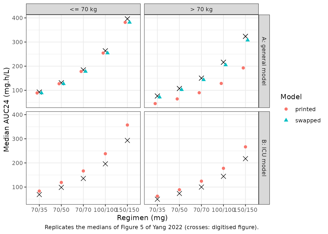
gen <- dplyr::filter(fig5_cmp, panel == "A: general model")
icu <- dplyr::filter(fig5_cmp, panel == "B: ICU model")
# Deterministic: no random draws. Below 70 kg both readings are the same model.
stopifnot(
  all(abs(gen$pct_diff[gen$wt_group == "<= 70 kg"]) < 10),
  all(abs(gen$pct_diff[gen$wt_group == "> 70 kg" & gen$reading == "swapped"]) < 10),
  # The printed weight effect halves the heavy group's AUC against the figure.
  all(gen$pct_diff[gen$wt_group == "> 70 kg" & gen$reading == "printed"] < -30)
)
# ICU panel: the heavy-to-light AUC ratio is 1 / 1.34 in the model.
icu_ratio <- icu |>
  dplyr::select(wt_group, dose, auc_fig) |>
  tidyr::pivot_wider(names_from = wt_group, values_from = auc_fig) |>
  dplyr::mutate(ratio = `<= 70 kg` / `> 70 kg`)
icu_ratio
#> # A tibble: 5 × 4
#>    dose `<= 70 kg` `> 70 kg` ratio
#>   <dbl>      <dbl>     <dbl> <dbl>
#> 1    35       68.9      49.7  1.39
#> 2    50       98.5      73.4  1.34
#> 3    70      136.      100    1.36
#> 4   100      196.      144.   1.36
#> 5   150      293.      218.   1.35
stopifnot(abs(median(icu_ratio$ratio) / 1.34 - 1) < 0.05)
Below 70 kg the general model reproduces Figure 5A to within 4%. Above 70 kg the printed coefficient gives AUCs about 40% below the figure, and the swapped reading reproduces it to within 6%. The figure’s heavy-to-light AUC ratio is 1.22, close to the swapped 1.24 and far from the printed 1.98.
In Figure 5B the ICU model’s weight effect is reproduced (heavy-to-light ratio 1.36 in the figure, 1.34 in the model), but the model’s AUC is about 22% above the figure in both weight groups: the figure implies a median clearance of about 0.51 L/h below 70 kg, against the printed theta1 of 0.42 L/h. The Discussion’s ‘typical CL 0.56 L/h in ICU patients with WT > 70 kg’ equals 0.42 x 1.34, which confirms the printed theta1; the source of the offset in Figure 5B is not stated.
Table S1 (probability of target attainment)
The PTA for C. albicans (free AUC24/MIC >= 20, unbound fraction 0.03) is the probability that CL <= Dose x 0.03 / (20 x MIC). It is computed without simulation for the 70/50 mg regimen.
pta_tab <- tidyr::expand_grid(wt = c(60, 80), mic = c(0.06, 0.12, 0.25)) |>
  dplyr::rowwise() |>
  dplyr::mutate(
    cl_max = 50 * 0.03 / (20 * mic),
    printed = 100 * mix_prob_below(
      cl_max, typ_gen$cl[typ_gen$WT == wt][order(typ_gen$ALB[typ_gen$WT == wt])],
      c(p_low_alb, 1 - p_low_alb), sd_gen
    ),
    swapped = 100 * mix_prob_below(
      cl_max, typ_swap$cl[typ_swap$WT == wt][order(typ_swap$ALB[typ_swap$WT == wt])],
      c(p_low_alb, 1 - p_low_alb), sd_gen
    )
  ) |>
  dplyr::ungroup()
pta_tab$table_s1 <- c(98.9, 89.1, 26.1, 99.5, 87.8, 2.3)
pta_tab |>
  dplyr::mutate(wt = ifelse(wt >= 70, "> 70 kg", "<= 70 kg"), mic = format(mic)) |>
  dplyr::select(wt, mic, table_s1, printed, swapped) |>
  dplyr::rename(
    "Weight" = wt, "MIC (mg/L)" = mic, "Table S1 PTA (%)" = table_s1,
    "Printed (%)" = printed, "Swapped (%)" = swapped
  ) |>
knitr::kable(digits = 1, caption = "PTA, 70/50 mg, C. albicans: Table S1 against the model.")| Weight | MIC (mg/L) | Table S1 PTA (%) | Printed (%) | Swapped (%) |
|---|---|---|---|---|
| <= 70 kg | 0.06 | 98.9 | 100.0 | 100.0 |
| <= 70 kg | 0.12 | 89.1 | 91.2 | 91.2 |
| <= 70 kg | 0.25 | 26.1 | 22.2 | 22.2 |
| > 70 kg | 0.06 | 99.5 | 91.7 | 99.8 |
| > 70 kg | 0.12 | 87.8 | 26.8 | 76.1 |
| > 70 kg | 0.25 | 2.3 | 0.2 | 8.2 |
At an MIC of 0.12 mg/L the printed coefficient gives a PTA of about 27% in patients above 70 kg, where Table S1 reports 87.8%; the swapped reading gives about 76%. Table S1 itself is not monotone in places (for example, its C. parapsilosis rows), so it is shown here but not used as a check of the weight effect.
Below 70 kg the two readings agree, and the whole C. albicans block of Table S1 there (five regimens, nine MICs) bears on how Table 3’s IIV percentages are read. Reading 29.2% as a CV (the model) or as 100 x omega gives a log-SD for CL of about 0.29; reading it as a variance would give sqrt(0.292) = 0.54.
s1_light <- data.frame(
  dose = rep(c(35, 50, 70, 100, 150), each = 9),
  mic = rep(c(0.008, 0.015, 0.03, 0.06, 0.12, 0.25, 0.5, 1, 2), 5),
  pta = c(
    100, 100, 100, 95.9, 71.2, 0.9, 0, 0, 0,
    100, 100, 100, 98.9, 89.1, 26.1, 0, 0, 0,
    100, 100, 100, 99.1, 96.7, 71.3, 0.9, 0, 0,
    100, 100, 100, 99.7, 98.3, 88.8, 26.6, 0, 0,
    100, 100, 100, 99.7, 99.6, 97.7, 75.4, 2.6, 0
  )
)
light_cl <- typ_gen$cl[typ_gen$WT == 60][order(typ_gen$ALB[typ_gen$WT == 60])]
rmse_for <- function(sd) {
  pred <- mapply(
    function(d, m) 100 * mix_prob_below(d * 0.03 / (20 * m), light_cl, c(p_low_alb, 1 - p_low_alb), sd),
    s1_light$dose, s1_light$mic
  )
  sqrt(mean((pred - s1_light$pta)^2))
}
omega_readings <- data.frame(
  reading = c("CV (model)", "100 x omega", "variance"),
  sd_cl = c(sd_gen, 0.292, sqrt(0.292))
)
omega_readings$rmse <- vapply(omega_readings$sd_cl, rmse_for, numeric(1))
omega_readings |>
  dplyr::rename("Reading of 29.2%" = reading, "log-SD of CL" = sd_cl, "RMSE against Table S1 (PTA points)" = rmse) |>
knitr::kable(digits = 3, caption = "Table S1, weight <= 70 kg, C. albicans: fit of each IIV reading.")| Reading of 29.2% | log-SD of CL | RMSE against Table S1 (PTA points) |
|---|---|---|
| CV (model) | 0.286 | 3.252 |
| 100 x omega | 0.292 | 3.268 |
| variance | 0.540 | 6.081 |
# Deterministic: the variance reading fits Table S1 far worse.
stopifnot(omega_readings$rmse[3] > 1.5 * omega_readings$rmse[1])
The variance reading is ruled out. The CV and 100 x omega readings differ by less than the precision of Table S1; the CV reading is kept.
Table 4 (mean individual clearance and AUC)
Table 4 reports a mean individual CL of 0.42 L/h for all 299 patients and 0.47 L/h for the hospital’s ICU patients, and mean AUCs of 126.46 and 101.46 mg.h/L. For a log-normal clearance, the expected mean CL is the typical value times exp(omega^2 / 2), and the expected mean of 50 mg / CL is 50 mg times the mean of 1 / CL_typical times exp(omega^2 / 2), each averaged over the covariate categories. The weight fractions are 25% for all patients (normal weights with the Table 1 mean and SD) and 15 of 51 for ICU patients (Supplementary 3.4.1).
cat_weights <- function(typ, p_alb, p_wt) {
  with(typ, ifelse(ALB < 35, p_alb, 1 - p_alb) * ifelse(WT >= 70, p_wt, 1 - p_wt))
}
expected_cl <- function(typ, p_alb, p_wt, sd) {
  sum(cat_weights(typ, p_alb, p_wt) * typ$cl) * exp(sd^2 / 2)
}
expected_auc <- function(typ, p_alb, p_wt, sd) {
  50 * sum(cat_weights(typ, p_alb, p_wt) / typ$cl) * exp(sd^2 / 2)
}
p_wt_all <- 1 - pnorm(70, 62.3, 11.5)
tab4 <- data.frame(
  group = c("All patients", "ICU patients"),
  published = c(0.42, 0.47),
  printed = c(
    expected_cl(typ_gen, 161 / 299, p_wt_all, sd_gen),
    expected_cl(typ_gen, 44 / 51, 15 / 51, sd_gen)
  ),
  swapped = c(
    expected_cl(typ_swap, 161 / 299, p_wt_all, sd_gen),
    expected_cl(typ_swap, 44 / 51, 15 / 51, sd_gen)
  ),
  published_auc = c(126.46, 101.46),
  printed_auc = c(
    expected_auc(typ_gen, 161 / 299, p_wt_all, sd_gen),
    expected_auc(typ_gen, 44 / 51, 15 / 51, sd_gen)
  ),
  swapped_auc = c(
    expected_auc(typ_swap, 161 / 299, p_wt_all, sd_gen),
    expected_auc(typ_swap, 44 / 51, 15 / 51, sd_gen)
  )
)
tab4 |>
  dplyr::rename(
    "Group" = group, "Table 4 CL (L/h)" = published,
    "Printed CL" = printed, "Swapped CL" = swapped,
    "Table 4 AUC (mg.h/L)" = published_auc,
    "Printed AUC" = printed_auc, "Swapped AUC" = swapped_auc
  ) |>
knitr::kable(digits = 3, caption = "Mean CL and AUC (50 mg daily), general model: Table 4 against the model.")| Group | Table 4 CL (L/h) | Printed CL | Swapped CL | Table 4 AUC (mg.h/L) | Printed AUC | Swapped AUC |
|---|---|---|---|---|---|---|
| All patients | 0.42 | 0.518 | 0.441 | 126.46 | 118.331 | 128.579 |
| ICU patients | 0.47 | 0.600 | 0.499 | 101.46 | 101.274 | 111.782 |
# Deterministic: for clearance, the swapped reading is the closer one in both groups.
stopifnot(all(abs(tab4$swapped - tab4$published) < abs(tab4$printed - tab4$published)))
The clearance column favours the swapped reading in both groups. The AUC column is mixed: the swapped reading fits all patients better and the printed reading fits the ICU patients better. The AUC column summarises each patient’s actual dose, which this calculation does not reproduce.
The printed coefficient also implies a typical CL of 0.32 x 1.46 x 1.98 = 0.925 L/h for a heavy, hypoalbuminaemic patient, above the largest individual CL in Table 4 (0.71 L/h).
The model keeps the printed values because no erratum or control
stream on record changes them. Users who want to reproduce the paper’s
dosing simulations can set e_wt_cl = 0.24 and
e_wt_vc = 0.98 with ini(), as above; the 0.98
on volume in that reading is inferred by symmetry and cannot be checked
against any published output.
Assumptions and deviations
-
Weight coefficients (general model). Table 3 is
encoded as printed (
e_wt_cl = 0.98,e_wt_vc = 0.24). Figure 5A, Table S1 and Table 4 fit the swapped assignment; see Weight coefficients. No erratum had been published when this model was added (checked 2026-10). - Dichotomised covariates. Albumin and weight enter only as indicators (albumin < 35 g/L; weight >= 70 kg), as in Table 3 footnote c. The figures and supplementary tables label the groups <= 70 / > 70 kg; the model follows the footnote’s >= 70 kg.
-
Structure. Results 3.2.1 calls the model
‘one-compartment … of first-order absorption and elimination’, but
caspofungin was infused over 1 h and no absorption rate is reported. The
model is a one-compartment model with infusion into
central. - Residual error. Methods 2.4 describes an exponential error model and Table 3 reports ‘Proportional (%)’. It is encoded as proportional, with the Table 3 percentage as the SD.
- IIV scale. Table 3 gives IIV in percent without a definition. It is read as a CV of a log-normal parameter, omega^2 = log(CV^2 + 1). Table S1 rules out reading it as a variance (see the PTA section); reading it as 100 x omega would give omega^2 of 0.085 and 0.350 instead of 0.082 and 0.300 for CL and V in the general model; in the ICU model both readings round to 0.018 and 0.038.
- ICU clearance. Table 3 gives theta1 = 0.42 L/h and the Abstract 0.40 L/h, which is the bootstrap mean. The table value is used; the Discussion’s 0.56 L/h above 70 kg (0.42 x 1.34) agrees with it.
- ICU residual error. The final estimate (24.3%) lies outside its own bootstrap 95% CI (28.6-34.1%). The estimate is used as printed.
- Figure 5B. The ICU panel implies a clearance about 22% above the ICU model’s theta1 in both weight groups (see above), and its boxes are wider than the model’s 13.5% IIV on CL would give: the interquartile ratio of the 150/150 mg box below 70 kg (about 360 / 234 mg.h/L) corresponds to a log-SD near 0.3. The paper’s ICU simulation therefore differs from the printed ICU model in ways the paper does not describe; the model is encoded as printed.
- Covariates held constant. Albumin and weight were recorded over the course of treatment; the virtual cohorts hold them constant, and the model accepts time-varying columns.
- Doses. Every virtual subject receives 70 mg then 50 mg daily; the patients’ 70/35 and 70/70 mg adjustments are not reproduced.
-
Excluded covariates. Cyclosporine,
methylprednisolone, ICU status and others were significant in forward
inclusion but removed in backward elimination (Table 2); they are listed
under
covariatesDataExcludedin the model files.