Erlotinib PK and NSCLC tumor dynamics with acquired resistance (Yin 2024)
Source:vignettes/articles/Yin_2024_erlotinib.Rmd
Yin_2024_erlotinib.RmdThe models
Yin et al. (2024) analysed erlotinib pharmacokinetics (PK) and the tumor dynamics of adults with EGFR-mutant non-small cell lung cancer (NSCLC). The paper reports three final models, each shipped as its own file:
| Model file | Content | Source |
|---|---|---|
Yin_2024_erlotinib |
Two-compartment popPK model, first-order absorption with a lag time, IIV on bioavailability | Table 2 |
Yin_2024_erlotinib_tumor |
Tumor-size (sum of longest diameters, SLD) model with a drug-sensitive and a drug-resistant clone, no covariate | Table 3 (left), Appendix S2 |
Yin_2024_erlotinib_tumor_ctdna |
The same tumor model with baseline plasma ctDNA EGFR variant allele frequency (VAF) on the growth rate | Table 3 (right), Appendix S2 |
The tumor model (Methods Eqs 1-4, Appendix S2) treats the tumor as a
drug-sensitive clone TS (state shrink), seeded
at the observed baseline SLD, and a drug-resistant clone TR
(state growth) that starts at zero:
- both clones grow first-order at a shared rate
kg(kge); - on treatment, the sensitive clone is killed first-order at
kd(kse) and converts to the resistant clone at the “mutation rate”km(kmut); - the observed SLD is
TS + TR.
The paper tested an exposure-dependent kill rate (linear and Emax on
the predicted erlotinib concentration) and did not retain it, so the
final tumor models have no PK input. Treatment enters
only through the on-treatment indicator TRT_PHASE (the
paper’s UNDERTREAT data column), which switches on the
kill, the conversion and the resistant clone’s growth. A model with
pre-existing (primary) resistance, TR_0 = 4.51 mm (Table
S1), did not improve the fit and is not shipped.
pk <- rxode2::rxode2(readModelDb("Yin_2024_erlotinib"))
#> ℹ parameter labels from comments will be replaced by 'label()'
tum <- rxode2::rxode2(readModelDb("Yin_2024_erlotinib_tumor"))
#> ℹ parameter labels from comments will be replaced by 'label()'
tumc <- rxode2::rxode2(readModelDb("Yin_2024_erlotinib_tumor_ctdna"))
#> ℹ parameter labels from comments will be replaced by 'label()'
Population
The PK model pooled two cohorts (Table 1): 29 patients with intensive steady-state profiles (13 samples each, predose to 24 h) from the control arms of two food-interaction studies at Erasmus MC (median age 63 years, 55% female, median weight 74 kg; 25 on 150 mg, 3 on 100 mg, 1 on 50 mg once daily), and 18 patients from the real-world START-TKI study (NCT05221372) who contributed 146 sparse samples (median age 66 years, 72% female, median weight 69.5 kg; all started at 150 mg once daily). The tumor models were fitted to the 155 SLD measurements (RECIST 1.1) of the 18 START-TKI patients, followed for a median of 264 days of treatment (range 20-1168), with a median baseline SLD of 76.6 mm (range 29-116). Baseline plasma ctDNA was available for 12 of the 18 patients; the median VAF of the primary EGFR variant was 1.74% (range 0-62.74%).
str(pk$meta$population[c("n_subjects", "age_range", "sex_female_pct", "dose_range")])
#> List of 4
#>  $ n_subjects    : num 45
#>  $ age_range     : chr "35-78 years"
#>  $ sex_female_pct: num 61.7
#>  $ dose_range    : chr "50-150 mg orally once daily (150 mg in 86% of the intensive cohort and all START-TKI patients)"
str(tum$meta$population[c("n_subjects", "age_range", "sex_female_pct", "notes")])
#> List of 4
#>  $ n_subjects    : num 18
#>  $ age_range     : chr "48-78 years"
#>  $ sex_female_pct: num 72.2
#>  $ notes         : chr "Yin 2024 Table 1 (PK/PD data, N = 18). 155 SLD measurements, median 7 per patient (range 2-18), over a median 2"| __truncated__
Source trace
| Quantity | Value | Source |
|---|---|---|
| PK: ka | 1.61 1/h | Table 2 |
| PK: CL/F | 4.10 L/h | Table 2 |
| PK: Vc/F | 142 L | Table 2 |
| PK: Vp/F | 2420 L | Table 2 |
| PK: Q/F | 0.548 L/h | Table 2 |
| PK: Tlag | 0.400 h | Table 2 |
| PK: F | 1 (fixed) | Table 2; Methods |
| PK: IIV CL/F, Vc/F, Q/F, ka, F | 15.7%, 20.3%, 194.4%, 124.5%, 16.3% CV | Table 2 |
| PK: proportional / additive error | 15.4% / 44.5 ng/mL | Table 2 |
| PK structure | 2-cmt, first-order absorption with lag, IIV on F | Results; Methods |
| Tumor: kg | 0.000799 1/day (no covariate); 0.00204 1/day (VAF >= 1.74%) | Table 3 |
| Tumor: f1, f2 (kg factor for VAF < 1.74%, VAF unavailable) | 0.334, 0.281 | Table 3 |
| Tumor: kd | 0.0121 / 0.0123 1/day | Table 3 |
| Tumor: km | 0.00911 / 0.00824 1/day | Table 3 |
| Tumor: IIV kg, kd, km | 60.3%, 68.4%, 56.5% CV / 16.6%, 66.2%, 57.9% CV | Table 3 |
| Tumor: proportional / additive error | 7.54% / 1.17 mm; 7.67% / 1.13 mm | Table 3 |
| Tumor: TS_0, TR_0 | observed baseline SLD, 0 (fixed) | Table 3 |
| Tumor ODEs and on-treatment gating |
UNDERTREAT multiplies kd, km and the resistant clone’s
growth |
Methods Eqs 1-4; Appendix S2 $DES
|
| Tumor time unit | day (PK rates converted with *24 in the tumor control
stream) |
Appendix S2 $PK
|
| ctDNA covariate cut |
baseVAF.GE.0.AND.baseVAF.LT.1.74; missing coded
negative |
Appendix S2 $PK
|
Pharmacokinetics
Virtual cohort and simulation
Two hundred virtual patients receive 150 mg erlotinib once daily (the dose of all START-TKI patients at the start of treatment). The model has no covariates. The observation window is the 14th dosing interval, 312-336 h. The very large, slowly equilibrating peripheral volume (Vp/F = 2420 L with Q/F = 0.548 L/h) means troughs keep rising slowly for months; see the steady-state check below.
rxode2::rxSetSeed(20240417)
n_pk <- 200
ev_pk <- rxode2::et(amt = 150, ii = 24, addl = 13, cmt = "depot") |>
  rxode2::et(seq(312, 336, by = 0.5), cmt = "central") |>
  rxode2::et(id = seq_len(n_pk))
sim_pk <- rxode2::rxSolve(pk, ev_pk, returnType = "data.frame") |>
  dplyr::mutate(treatment = "150 mg QD", tad = time - 312)
Replicating Figure 2
sim_pk |>
  dplyr::group_by(tad) |>
  dplyr::summarise(
    p05 = quantile(Cc, 0.05), p50 = median(Cc), p95 = quantile(Cc, 0.95),
    .groups = "drop"
  ) |>
  ggplot(aes(tad, p50)) +
  geom_ribbon(aes(ymin = p05, ymax = p95), alpha = 0.25, fill = "steelblue") +
  geom_line(colour = "firebrick", linewidth = 1) +
  labs(x = "Time after last dose (h)", y = "Erlotinib concentration (ng/mL)") +
  theme_bw()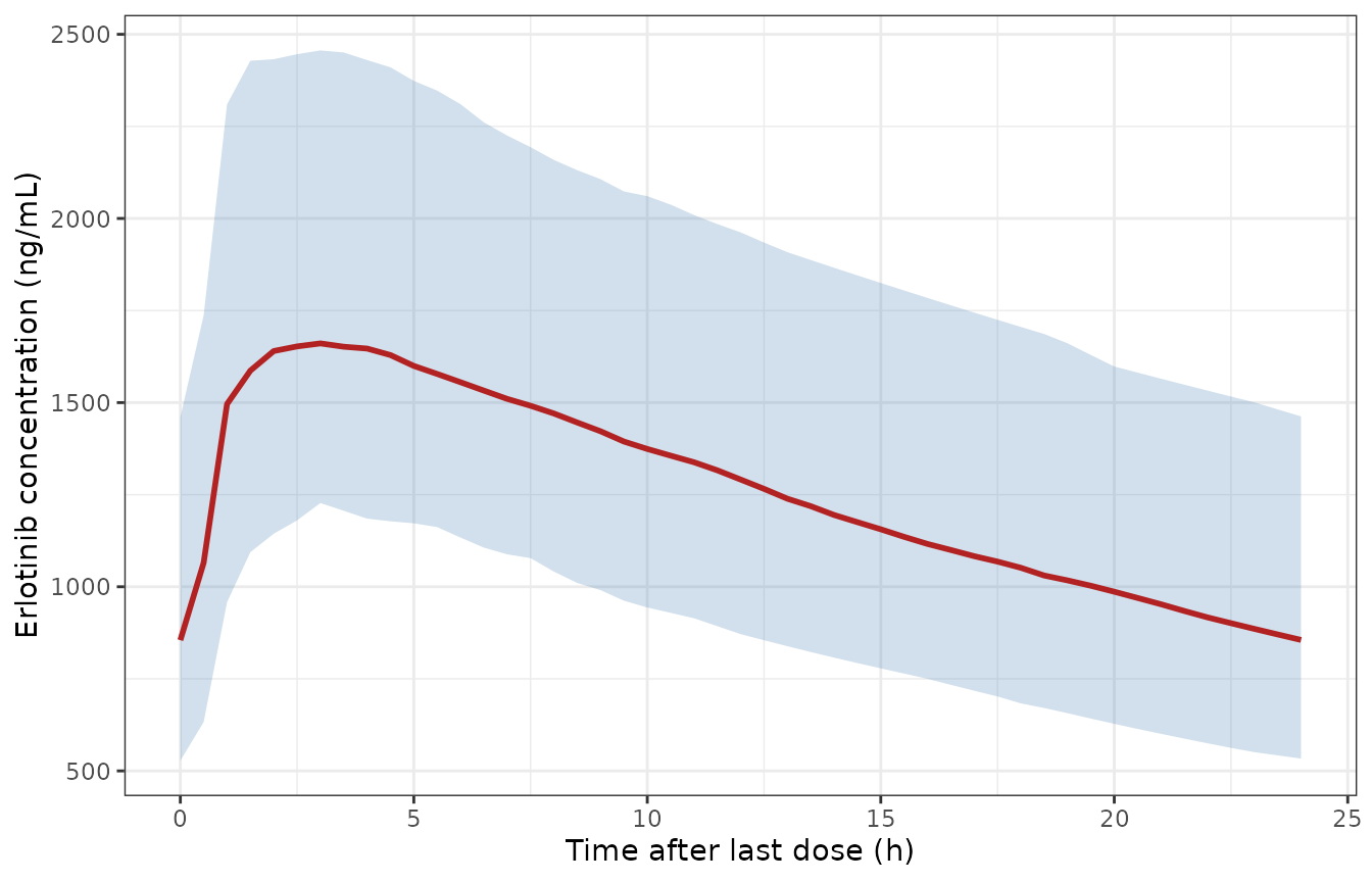
Simulated steady-state erlotinib concentrations versus time after dose (median and 5th-95th percentiles of 200 virtual patients, 150 mg once daily, day 14). Replicates Figure 2 of Yin 2024, whose observed median peaks near 1700 ng/mL at 2-3 h and falls to about 850 ng/mL at 24 h.
PKNCA
conc_pk <- sim_pk |>
  dplyr::filter(!is.na(Cc)) |>
  dplyr::select(id, time, Cc, treatment)
dose_pk <- data.frame(id = seq_len(n_pk), time = 312, amt = 150, treatment = "150 mg QD")

o_conc <- PKNCA::PKNCAconc(conc_pk, Cc ~ time | treatment + id)
o_dose <- PKNCA::PKNCAdose(dose_pk, amt ~ time | treatment + id)
intervals <- data.frame(
  start = 312, end = 336,
  cmax = TRUE, tmax = TRUE, cmin = TRUE, auclast = TRUE
)
nca_pk <- PKNCA::pk.nca(PKNCA::PKNCAdata(o_conc, o_dose, intervals = intervals))
summary(nca_pk)
#>  start end treatment   N      auclast        cmax       cmin              tmax
#>    312 336 150 mg QD 200 31100 [24.8] 1760 [22.0] 868 [32.4] 2.50 [1.00, 10.0]
#>
#> Caption: auclast, cmax, cmin: geometric mean and geometric coefficient of variation; tmax: median and range; N: number of subjects
Comparison against published values
The paper does not report NCA. Two summary values are available: the median of the 125 START-TKI trough concentrations taken at least 20 h after the last dose (842 ng/mL, Results), and the median observed peak of Figure 2 (about 1700 ng/mL at 2-3 h, digitised by the maintainers).
published_pk <- data.frame(treatment = "150 mg QD", cmin = 842, cmax = 1700)
cmp_pk <- nlmixr2lib::ncaComparisonTable(
  simulated = nca_pk,
  reference = published_pk,
  by = "treatment",
  params = c("cmax", "cmin"),
  units = c(cmax = "ng/mL", cmin = "ng/mL"),
  tolerance_pct = 20
)
knitr::kable(cmp_pk, caption = attr(cmp_pk, "footnote"))| NCA parameter | treatment | Reference | Simulated | % diff |
|---|---|---|---|---|
| Cmax (ng/mL) | 150 mg QD | 1700 | 1710 | +0.6% |
| Cmin (ng/mL) | 150 mg QD | 842 | 855 | +1.5% |
sim_med <- as.data.frame(nca_pk$result) |>
  dplyr::filter(PPTESTCD %in% c("cmin", "cmax")) |>
  dplyr::group_by(PPTESTCD) |>
  dplyr::summarise(med = median(PPORRES), .groups = "drop")
stopifnot(
  # A mis-transcribed CL/F, Vc/F or ng/mL scaling shifts these by far more
  # than 25%; the comparison is to an observed median, not a model output.
  abs(sim_med$med[sim_med$PPTESTCD == "cmin"] / 842 - 1) < 0.25,
  abs(sim_med$med[sim_med$PPTESTCD == "cmax"] / 1700 - 1) < 0.25
)
The observed troughs came from real-world patients, some on reduced doses (75-150 mg) and at varying times after the start of treatment, and the Figure 2 peak is read off a plot. The simulated medians agree with both to within a few percent, which is closer than these comparisons can resolve; the assertion above therefore uses a 25% band.
Steady-state exposure
At true steady state the typical AUC over a dosing interval equals
F * Dose / (CL/F) = 150 mg / 4.10 L/h = 36.6 mg h/L. The
slow peripheral compartment needs months to fill, so the typical AUC
reaches 89% of that value on day 14 and 98% on day 400.
pk_typ <- rxode2::zeroRe(pk)
auc_tau <- function(day) {
  t0 <- (day - 1) * 24
  ev <- rxode2::et(amt = 150, ii = 24, addl = day - 1, cmt = "depot") |>
    rxode2::et(seq(t0, t0 + 24, by = 0.25), cmt = "central")
  s <- rxode2::rxSolve(pk_typ, ev, returnType = "data.frame")
  s <- s[s$time >= t0, ]
  sum(diff(s$time) * (head(s$Cc, -1) + tail(s$Cc, -1)) / 2)
}
auc_ss <- 150 / 4.10 * 1000
ss_tab <- data.frame(day = c(14, 100, 400)) |>
  dplyr::mutate(
    auc = vapply(day, auc_tau, numeric(1)),
    fraction_of_ss = auc / auc_ss
  )
#> ℹ omega/sigma items treated as zero: 'etalcl', 'etalvc', 'etalq', 'etalka', 'etalfdepot'
#> ℹ omega/sigma items treated as zero: 'etalcl', 'etalvc', 'etalq', 'etalka', 'etalfdepot'
#> ℹ omega/sigma items treated as zero: 'etalcl', 'etalvc', 'etalq', 'etalka', 'etalfdepot'
ss_tab |>
  dplyr::rename(
    "Dosing day" = day,
    "Typical AUC0-24 (ng*h/mL)" = auc,
    "Fraction of Dose/CL" = fraction_of_ss
  ) |>
knitr::kable(digits = 3)| Dosing day | Typical AUC0-24 (ng*h/mL) | Fraction of Dose/CL |
|---|---|---|
| 14 | 32504.76 | 0.888 |
| 100 | 33884.25 | 0.926 |
| 400 | 35946.56 | 0.983 |
Tumor dynamics
The ODE solution matches the closed form
With treatment on from time 0 and TR(0) = 0, the
equations solve to TS(t) = TS0 exp(a t) and
TR(t) = TS0 km / (kd + km) (exp(kg t) - exp(a t)) with
a = kg - kd - km. Both sides use the same parameters, so
the difference is solver error only.
tum_typ <- rxode2::zeroRe(tum)
grid <- seq(0, 1200, by = 10)
d_typ <- data.frame(
  id = 1, time = grid, evid = 0, amt = 0, cmt = "shrink",
  TUM_SLD = 76.6, TRT_PHASE = 1
)
s_typ <- rxode2::rxSolve(tum_typ, d_typ, returnType = "data.frame")
#> ℹ omega/sigma items treated as zero: 'etalkge', 'etalkse', 'etalkmut'
kg <- 0.000799
kd <- 0.0121
km <- 0.00911
a <- kg - kd - km
closed <- 76.6 * exp(a * grid) + 76.6 * km / (kd + km) * (exp(kg * grid) - exp(a * grid))
stopifnot(max(abs(s_typ$TS / closed - 1)) < 1e-5)
t_nadir <- log((kd + km - kg) * kd / (km * kg)) / (kd + km)
t_nadir
#> [1] 166.1622

nadir <- s_typ[which.min(s_typ$TS), ]
c(nadir_day = nadir$time, nadir_mm = nadir$TS, pct_change = 100 * (nadir$TS / 76.6 - 1))
#>  nadir_day   nadir_mm pct_change
#>  170.00000   39.04741  -49.02427
Setting the derivative of the closed form to zero gives the typical
time of the nadir,
t = log((kd + km - kg) * kd / (km * kg)) / (kd + km) = 166
days, with a 49% reduction from a 76.6 mm baseline. That agrees with the
Figure 3 median, which reaches roughly 30-45 mm between days 150 and
400.
Treatment gating
Before treatment starts (TRT_PHASE = 0) the sensitive
clone grows at kg alone and the resistant clone stays at
zero. Starting treatment on day 60:
d_gate <- data.frame(
  id = 1, time = seq(0, 300, by = 5), evid = 0, amt = 0, cmt = "shrink",
  TUM_SLD = 76.6
) |>
  dplyr::mutate(TRT_PHASE = as.integer(time >= 60))
s_gate <- rxode2::rxSolve(tum_typ, d_gate, returnType = "data.frame")
#> ℹ omega/sigma items treated as zero: 'etalkge', 'etalkse', 'etalkmut'
pre <- s_gate[s_gate$time <= 60, ]
stopifnot(
  max(abs(pre$TS / (76.6 * exp(kg * pre$time)) - 1)) < 1e-6,
  all(pre$growth[pre$time < 60] == 0)
)
Replicating Figure 3
rxode2::rxSetSeed(20240418)
n_tum <- 200
# Baseline SLD log-normal around the cohort median 76.6 mm, kept to the
# observed 29-116 mm range.
base_sld <- pmin(pmax(exp(rnorm(n_tum, log(76.6), 0.35)), 29), 116)
d_vpc <- tidyr::expand_grid(id = seq_len(n_tum), time = seq(0, 1200, by = 20)) |>
  dplyr::mutate(
    evid = 0, amt = 0, cmt = "shrink",
    TUM_SLD = base_sld[id], TRT_PHASE = 1
  )
s_vpc <- rxode2::rxSolve(tum, d_vpc, returnType = "data.frame")
vpc <- s_vpc |>
  dplyr::group_by(time) |>
  dplyr::summarise(
    p05 = quantile(TS, 0.05), p50 = median(TS), p95 = quantile(TS, 0.95),
    .groups = "drop"
  )
ggplot(vpc, aes(time, p50)) +
  geom_ribbon(aes(ymin = p05, ymax = p95), alpha = 0.25, fill = "steelblue") +
  geom_line(colour = "firebrick", linewidth = 1) +
  labs(x = "Time (days)", y = "Sum of longest diameters (mm)") +
  theme_bw()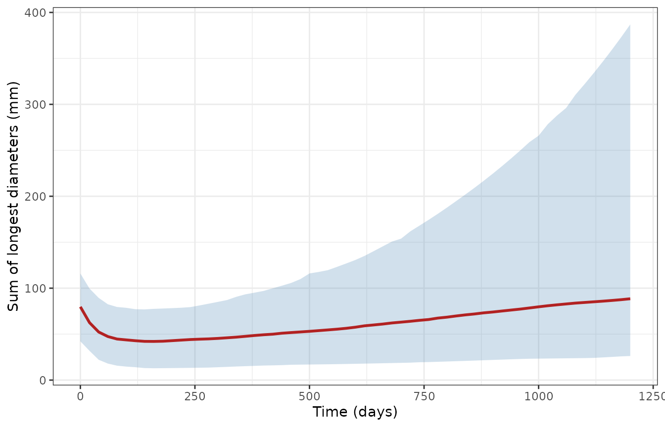
Simulated SLD (median and 5th-95th percentiles of 200 virtual patients, treatment from day 0). Replicates the simulation intervals of Figure 3 of Yin 2024; the paper’s VPC also simulated progression-related dropout, which this simulation does not, so its upper band rises later and higher than the published one.
The ctDNA covariate model
The typical growth rate depends on the baseline VAF of the primary
EGFR variant (Table 3; Results): kg = 0.00204 1/day for VAF
>= 1.74%, 0.334 * 0.00204 for VAF < 1.74% (including
no detectable variant), and 0.281 * 0.00204 when no
baseline sample was available.
tumc_typ <- rxode2::zeroRe(tumc)
grp <- data.frame(
  group = c("VAF >= 1.74%", "VAF < 1.74%", "VAF unavailable"),
  CTDNA_VAF = c(10, 0.5, 0),
  CTDNA_VAF_MISSING = c(0, 0, 1),
  kg_expected = 0.00204 * c(1, 0.334, 0.281)
)
d_grp <- tidyr::expand_grid(id = 1:3, time = seq(0, 1200, by = 10)) |>
  dplyr::mutate(
    evid = 0, amt = 0, cmt = "shrink", TUM_SLD = 76.6, TRT_PHASE = 1,
    CTDNA_VAF = grp$CTDNA_VAF[id], CTDNA_VAF_MISSING = grp$CTDNA_VAF_MISSING[id]
  )
# One typical-value solve per group (a multi-subject solve of a zeroRe()
# model warns that there is no omega).
s_grp <- lapply(1:3, function(i) {
  rxode2::rxSolve(tumc_typ, d_grp[d_grp$id == i, ], returnType = "data.frame") |>
    dplyr::mutate(id = i)
}) |>
  dplyr::bind_rows()
#> ℹ omega/sigma items treated as zero: 'etalkge', 'etalkse', 'etalkmut'
#> ℹ omega/sigma items treated as zero: 'etalkge', 'etalkse', 'etalkmut'
#> ℹ omega/sigma items treated as zero: 'etalkge', 'etalkse', 'etalkmut'
kg_sim <- s_grp |>
  dplyr::group_by(id) |>
  dplyr::summarise(kg_sim = dplyr::first(kge), .groups = "drop")
stopifnot(max(abs(kg_sim$kg_sim / grp$kg_expected - 1)) < 1e-12)

# The cut is at 1.74% with 1.74% itself in the reference group (Appendix S2).
d_edge <- d_grp[d_grp$id == 1, ] |> dplyr::mutate(CTDNA_VAF = 1.74)
s_edge <- rxode2::rxSolve(tumc_typ, d_edge, returnType = "data.frame")
#> ℹ omega/sigma items treated as zero: 'etalkge', 'etalkse', 'etalkmut'
stopifnot(abs(s_edge$kge[1] / 0.00204 - 1) < 1e-12)
s_grp |>
  dplyr::mutate(group = factor(grp$group[id], levels = grp$group)) |>
  ggplot(aes(time, TS, colour = group)) +
  geom_line(linewidth = 1) +
  labs(x = "Time (days)", y = "Sum of longest diameters (mm)", colour = NULL) +
  theme_bw()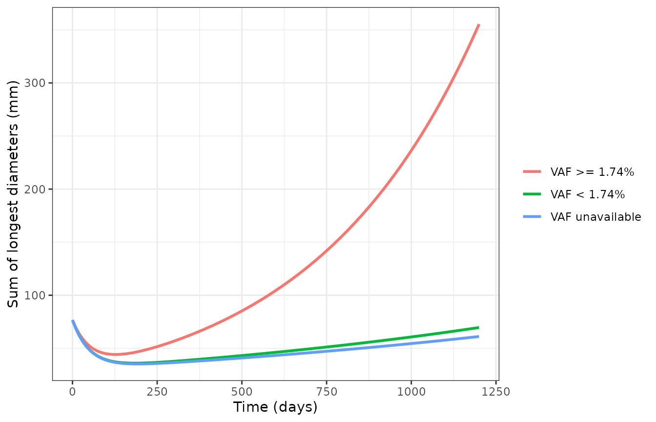
Typical SLD by baseline plasma EGFR VAF category (76.6 mm baseline), ctDNA covariate model. Higher baseline EGFR VAF gives faster growth and earlier regrowth (Yin 2024 Results).
nadirs <- s_grp |>
  dplyr::group_by(id) |>
  dplyr::slice_min(TS, n = 1, with_ties = FALSE) |>
  dplyr::ungroup() |>
  dplyr::mutate(group = grp$group[id]) |>
  dplyr::select(group, nadir_day = time, nadir_mm = TS)
knitr::kable(
  nadirs |> dplyr::rename("Baseline VAF" = group, "Nadir day" = nadir_day, "Nadir SLD (mm)" = nadir_mm),
  digits = 1
)| Baseline VAF | Nadir day | Nadir SLD (mm) |
|---|---|---|
| VAF >= 1.74% | 130 | 44.2 |
| VAF < 1.74% | 180 | 36.0 |
| VAF unavailable | 190 | 35.3 |
stopifnot(
  # Faster growth in the high-VAF group: earlier and shallower nadir.
  nadirs$nadir_day[1] < nadirs$nadir_day[2],
  nadirs$nadir_mm[1] > nadirs$nadir_mm[2]
)
Assumptions and deviations
-
IIV scale. Tables 2 and 3 report IIV as CV%. The
variances are
omega^2 = log(1 + CV^2); the paper does not state the conversion it used. For the large PK IIVs (Q/F 194.4%, ka 124.5%) the alternative readingomega = CVwould give much larger variances (3.78 and 1.55 rather than 1.56 and 0.94). -
Residual error. The tumor control stream uses
W = sqrt(THETA(3)^2 * IPRED^2 + THETA(4)^2)withSIGMA 1 FIX, which is nlmixr2’s combined (variance-sum) additive + proportional error. The PK model’s error code is not published; Methods describes the same combined form, and it is encoded the same way. -
Reported rate units. The tumor control stream
divides each
THETAby 100 (KG1 = THETA(1)*EXP(ETA(1))/100). The Table 3 values (for example kg = 0.000799 1/day) lie within the scaled bounds of the$THETAblock, so they are taken as the rates after that scaling. - Tumor files are separate from the PK file. The tumor control stream carries the PK compartments only so that concentrations “can be simulated, if needed”; no tumor parameter depends on them in the final models, so the tumor files contain only the two tumor states. Time is in days in the tumor files and in hours in the PK file.
-
Treatment indicator.
UNDERTREATmaps to theTRT_PHASEcolumn. As in the paper, it also gates the resistant clone’s growth, which has no effect while that clone is zero before treatment. After treatment stops, the data were censored, so the models say nothing about regrowth off treatment. -
ctDNA cut. Table 3 and the control stream use
VAF < 1.74%; parts of the Results text say “less than or equal to 1.74%”. The control stream’s strict inequality is encoded, so a VAF of exactly 1.74% is in the reference group. Subjects without a baseline sample takeCTDNA_VAF_MISSING = 1and any finiteCTDNA_VAF(0 is used here). - Not shipped. The primary-resistance variant (Table S1) and the exposure-dependent kill-rate variants were tested and not retained. Baseline TP53 mutation status and baseline cfDNA concentration were tested as covariates and were not significant.
- Validation targets. The paper reports no NCA. The PK comparison uses the observed median trough from the Results and a median peak digitised by the maintainers from Figure 2. The tumor VPC is compared qualitatively with Figure 3, which included simulated dropout.