Pexidartinib (Yin 2020)
Source:vignettes/articles/Yin_2020_pexidartinib.Rmd
Yin_2020_pexidartinib.RmdModel and source
- Citation: Yin O, Kang J, Knebel W, Zahir H, van de Sande M, Tap WD, Gelderblom H, Stacchiotti S, Greenberg J, Shuster D, Wagner AJ. Population Pharmacokinetic Analysis of Pexidartinib in Healthy Subjects and Patients With Tenosynovial Giant Cell Tumor or Other Solid Tumors. J Clin Pharmacol. 2021 Apr;61(4):480-492. doi:10.1002/jcph.1753. PDF on disk: ACoP 2019 poster of the same analysis (metrum_nd_pexidartinib_healthy.pdf).
- Description: Two-compartment population PK model for oral pexidartinib (CSF1R/KIT/FLT3 inhibitor) in healthy subjects and adult patients with tenosynovial giant cell tumour (TGCT) or other advanced solid tumours (Yin 2020). Absorption is sequential zero-order deposition into a depot (duration D1, lag time ALAG1) followed by first-order absorption (KA) into the central compartment, with linear elimination from central. Apparent clearance CL/F scales allometrically on (WT/80)^0.75 and is additionally modified by piecewise power effects of CRCL (active only when CRCL < 90 mL/min), AST (active only when AST > 80 U/L), and total bilirubin (active only when TBILI > 20.5 umol/L), plus multiplicative effects for Asian race (1.27x), healthy-participant cohort (1.26x; the Phase 1 healthy-subject studies), and female sex (0.869x). Apparent central and peripheral volumes Vc/F and Vp/F scale on (WT/80)^1; apparent inter-compartmental clearance Q/F scales on (WT/80)^0.75. Relative bioavailability of the Phase 1 formulation is fixed at 0.855 vs the Phase 3 / commercial reference formulation. Inter-individual variability is a 3x3 block on log(CL,Vc,Vp), independent diagonals on log(KA) and log(Q), and a Phase-1-formulation-specific IIV on the F1 bioavailability anchor. The published inter-occasion variability (5 occasions on KA, 10 occasions on F1) is not encoded structurally here (following the Andrews 2017 / Brooks 2021 tacrolimus precedent for the model-library use case where no operational occasion column is defined). Residual error is proportional with separate magnitudes for patient samples (29.7% CV) and healthy-subject samples (19.6% CV), switched per-subject by the DIS_HEALTHY indicator.
- Article: https://doi.org/10.1002/jcph.1753
- ACoP 2019 poster (PDF on disk for this extraction): https://metrumrg.com/wp-content/uploads/2019/11/ACoP2019-PopK-Pexi.pdf
Yin et al. (2020) developed a population pharmacokinetic model for oral pexidartinib (CSF1R / KIT / FLT3 inhibitor; FDA-approved as Turalio for adult tenosynovial giant cell tumour) pooled across 375 subjects in nine clinical studies: seven Phase 1 clinical pharmacology studies in 159 healthy subjects (relative bioavailability, dose proportionality, drug-drug interaction with itraconazole / rifampin / esomeprazole, and food effect; single doses 200-2400 mg), the Phase 1 PLX108-01 dose-ranging study in 132 patients with TGCT or other advanced solid tumours (200-1200 mg/day), and the Phase 3 ENLIVEN (PLX108-10) study in 84 patients with TGCT (Part 1: 1000 mg/day for two weeks then 800 mg/day; Part 2: 800 mg/day). The structural model is a two-compartment model with sequential zero- and first-order absorption, an absorption lag time, and linear elimination from the central compartment. The covariate model retained body weight (on CL/F and Q/F at the theory-based 0.75 exponent; on Vc/F and Vp/F at exponent 1), piecewise effects of creatinine clearance, AST, and total bilirubin on CL/F, multiplicative effects of Asian race, healthy-participant cohort, and female sex on CL/F, and a fixed Phase 1 vs Phase 3 formulation effect on bioavailability. This vignette reproduces the typical-value structural model, simulates the ENLIVEN 800 mg/day (400 mg BID) regimen at steady state, and validates the simulated NCA outputs against the post hoc NCA parameters published in Yin 2020 Table 3.
Population
The pooled analysis cohort (Yin 2020 Methods Table 1) was N = 375 subjects contributing 8430 PK samples: 159 adult healthy subjects in seven Phase 1 clinical pharmacology studies (U114, U116, U117, U118, U119, U120, U121; single doses 200-2400 mg), 132 patients in PLX108-01 (Phase 1 dose-ranging in TGCT and other solid tumours, 200-1200 mg/day), and 84 patients in PLX108-10 ENLIVEN (Phase 3 in TGCT; Part 1: 1000 mg/day for two weeks followed by 800 mg/day; Part 2: 800 mg/day). Eight subjects (2.1%) were Asian and the remaining 367 (97.9%) were non-Asian. The reference subject in Yin 2020 Figure 2 (covariate forest plot) is a male, non-Asian patient with body weight 80 kg (the cohort median), creatinine clearance >= 90 mL/min, AST <= 80 U/L, and total bilirubin <= 20.5 umol/L. Pexidartinib serum concentrations were measured by a validated LC-MS/MS method with LLOQ 2.5 ng/mL.
The same information is available programmatically via the model’s
population metadata
(rxode2::rxode(readModelDb("Yin_2020_pexidartinib"))$meta$population).
Source trace
The per-parameter origin is recorded as an in-file comment next to
each ini() entry in
inst/modeldb/specificDrugs/Yin_2020_pexidartinib.R. The
table below collects them in one place for review.
| Equation / parameter | Value | Source location |
|---|---|---|
lcl (CL/F) |
log(5.83) (L/hr) | Yin 2020 Table 2: CL/F exp(theta1) = 5.83 (95% CI 5.43-6.27) |
lvc (Vc/F) |
log(98.0) (L) | Yin 2020 Table 2: Vc/F exp(theta2) = 98.0 (95% CI 90.0-107) |
lvp (Vp/F) |
log(116) (L) | Yin 2020 Table 2: Vp/F exp(theta3) = 116 (95% CI 106-128) |
lq (Q/F) |
log(20.7) (L/hr) | Yin 2020 Table 2: Q/F exp(theta4) = 20.7 (95% CI 17.9-23.8) |
lka (KA) |
log(6.82) (1/hr) | Yin 2020 Table 2: KA exp(theta5) = 6.82 (95% CI 5.09-9.14) |
ltlag (ALAG1) |
log(0.387) (hr) | Yin 2020 Table 2: ALAG1 exp(theta6) = 0.387 (95% CI 0.385-0.390) |
ld1 (D1) |
log(1.22) (hr) | Yin 2020 Table 2: D1 exp(theta7) = 1.22 (95% CI 1.20-1.25) |
lfdepot (F1 Phase 1) |
fixed(log(0.855)) | Yin 2020 Table 2: F1 Phase1 exp(theta8) = 0.855 Fixed |
e_wt_cl |
fixed(0.75) | Yin 2020 Table 2 row 1 trailing exponent |
e_wt_vc |
fixed(1) | Yin 2020 Table 2 row 8 trailing exponent |
e_wt_vp |
fixed(1) | Yin 2020 Table 2 row 9 trailing exponent |
e_wt_q |
fixed(0.75) | Yin 2020 Table 2 row 10 trailing exponent |
e_crcl_cl (piecewise CRCL < 90) |
-0.0941 | Yin 2020 Table 2: theta9 (95% CI -0.402, 0.214) |
e_asian_cl |
1.27 | Yin 2020 Table 2: exp(theta10) (95% CI 1.05-1.54) |
e_ast_cl (piecewise AST > 80) |
0.0709 | Yin 2020 Table 2: theta11 (95% CI -0.180, 0.322) |
e_tbili_cl (piecewise TBILI > 20.5) |
0.244 | Yin 2020 Table 2: theta12 (95% CI 0.183-0.306) |
e_healthy_cl |
1.26 | Yin 2020 Table 2: exp(theta13) (95% CI 1.16-1.36) |
e_female_cl |
0.869 | Yin 2020 Table 2: exp(theta14) (95% CI 0.808-0.934) |
| IIV CL/F (Omega 1.1) | 0.0860 (30.0% CV) | Yin 2020 Table 2 final-model Omega matrix |
| IIV Vc/F (Omega 2.2) and cov(Vc,CL) (Omega 2.1) | 0.274 / 0.0774 (corr 0.504) | Yin 2020 Table 2 final-model Omega matrix |
| IIV Vp/F (Omega 3.3), cov(Vp,CL) (Omega 3.1), cov(Vp,Vc) (Omega 3.2) | 0.213 / 0.0149 / -0.0467 | Yin 2020 Table 2 final-model Omega matrix |
| IIV Q/F (Omega 4.4) | 0.406 (70.8% CV) | Yin 2020 Table 2 final-model Omega matrix |
| IIV KA (Omega 5.5) | 1.31 (165% CV) | Yin 2020 Table 2 final-model Omega matrix |
| IIV Phase 1 F1 (Omega 6.6) | 0.101 (32.6% CV) | Yin 2020 Table 2 final-model Omega matrix; gated by FORM_PEX_PHASE1 |
propSd_patient |
sqrt(0.0883) = 0.297 | Yin 2020 Table 2 Sigma 1.1 prop pat (29.7% CV) |
propSd_healthy |
sqrt(0.0384) = 0.196 | Yin 2020 Table 2 Sigma 2.2 prop ht (19.6% CV) |
| Reference body weight | 80 kg | Yin 2020 Figure 2 caption (cohort median) |
| Reference CRCL threshold | 90 mL/min | Yin 2020 Table 2 row 2 piecewise denominator |
| Reference AST threshold | 80 U/L | Yin 2020 Table 2 row 4 piecewise denominator |
| Reference TBILI threshold | 20.5 umol/L | Yin 2020 Table 2 row 5 piecewise denominator |
| Sequential ZO + FO absorption ODE structure | d/dt(depot), d/dt(central), d/dt(peripheral1),
dur(depot) = d1, alag(depot) = tlag
|
Yin 2020 Methods, “two-compartment model with sequential zero- and first-order absorption and lag time” |
Virtual cohort
The ENLIVEN Phase 3 trial concentration-time data are not publicly available. The validation cohort below is a virtual replicate of the ENLIVEN study population: 200 adult patients with TGCT receiving the approved 800 mg/day Turalio regimen (400 mg BID), Phase 3 commercial formulation, with baseline covariate distributions chosen to bracket the Yin 2020 Figure 2 reference values.
set.seed(20260624)

n_patient <- 200L

cohort <- tibble::tibble(
  id              = seq_len(n_patient),
  WT              = exp(rnorm(n_patient, log(80), 0.18)),          # log-normal around 80 kg, ~20% CV
  SEXF            = rbinom(n_patient, 1, 0.5),                     # 50% female
  RACE_ASIAN      = rbinom(n_patient, 1, 8 / 375),                 # 2.1% Asian, matching Yin 2020 pooled cohort
  CRCL            = pmax(exp(rnorm(n_patient, log(110), 0.22)), 40),  # mostly above 90 mL/min, floor 40
  AST             = exp(rnorm(n_patient, log(25), 0.45)),          # mostly below 80 U/L
  TBILI           = exp(rnorm(n_patient, log(8), 0.40)),           # mostly below 20.5 umol/L
  DIS_HEALTHY     = 0L,                                            # TGCT patient cohort
  FORM_PEX_PHASE1 = 0L                                             # Phase 3 commercial formulation
)
summary(cohort[, c("WT", "CRCL", "AST", "TBILI")])
#>        WT              CRCL             AST             TBILI
#>  Min.   : 49.85   Min.   : 50.37   Min.   : 5.704   Min.   : 2.297
#>  1st Qu.: 71.71   1st Qu.: 96.08   1st Qu.:18.316   1st Qu.: 6.210
#>  Median : 80.87   Median :110.67   Median :25.028   Median : 8.147
#>  Mean   : 82.00   Mean   :111.24   Mean   :27.786   Mean   : 8.917
#>  3rd Qu.: 91.57   3rd Qu.:124.83   3rd Qu.:33.825   3rd Qu.:11.000
#>  Max.   :128.21   Max.   :196.36   Max.   :95.016   Max.   :20.208

# Build the event table: 400 mg Q12h dosing for 56 days, with rich PK sampling
# on Day 1 (0-12 h) and Day 56 (1332-1344 h) bracketing the AUC0-12 windows
# reported in Yin 2020 Table 3.
n_days       <- 56L
dose_mg      <- 400
ii_h         <- 12
day1_obs     <- c(0, 0.25, 0.5, 0.75, 1, 1.5, 2, 3, 4, 6, 8, 10, 12)
day56_anchor <- (n_days - 1L) * 24                                  # last full SS dose at t = 1332 h
day56_obs    <- day56_anchor + c(0, 0.25, 0.5, 0.75, 1, 1.5, 2, 3, 4, 6, 8, 10, 12)

make_subject_events <- function(subj_row) {
  doses <- tibble::tibble(
    id   = subj_row$id,
    time = seq(0, (n_days * 24) - ii_h, by = ii_h),
    evid = 1L,
    amt  = dose_mg,
    cmt  = "depot"
  )
  obs <- tibble::tibble(
    id   = subj_row$id,
    time = c(day1_obs, day56_obs),
    evid = 0L,
    amt  = 0,
    cmt  = "central"
  )
  rows <- dplyr::bind_rows(doses, obs)
  rows$WT              <- subj_row$WT
  rows$SEXF            <- subj_row$SEXF
  rows$RACE_ASIAN      <- subj_row$RACE_ASIAN
  rows$CRCL            <- subj_row$CRCL
  rows$AST             <- subj_row$AST
  rows$TBILI           <- subj_row$TBILI
  rows$DIS_HEALTHY     <- subj_row$DIS_HEALTHY
  rows$FORM_PEX_PHASE1 <- subj_row$FORM_PEX_PHASE1
  rows
}

events <- cohort |>
  split(seq_len(n_patient)) |>
  lapply(function(r) make_subject_events(as.list(r))) |>
  dplyr::bind_rows() |>
  dplyr::arrange(id, time, dplyr::desc(evid))
stopifnot(!anyDuplicated(unique(events[, c("id", "time", "evid")])))
nrow(events)
#> [1] 27600
Simulation
mod <- readModelDb("Yin_2020_pexidartinib")

sim <- rxode2::rxSolve(mod, events = events) |>
  as.data.frame() |>
  dplyr::filter(time %in% c(day1_obs, day56_obs))
#> ℹ parameter labels from comments will be replaced by 'label()'
nrow(sim)
#> [1] 5200
Day 1 vs steady-state concentration-time profiles
sim |>
  dplyr::mutate(
    phase     = ifelse(time <= 12, "Day 1 (first dose)", "Day 56 (steady state)"),
    time_dose = ifelse(time <= 12, time, time - day56_anchor)
  ) |>
  dplyr::group_by(phase, time_dose) |>
  dplyr::summarise(
    Q05 = quantile(Cc, 0.05, na.rm = TRUE),
    Q50 = quantile(Cc, 0.50, na.rm = TRUE),
    Q95 = quantile(Cc, 0.95, na.rm = TRUE),
    .groups = "drop"
  ) |>
  ggplot(aes(time_dose, Q50)) +
  geom_ribbon(aes(ymin = Q05, ymax = Q95), alpha = 0.25) +
  geom_line() +
  facet_wrap(~phase, scales = "free_y") +
  labs(x = "Time after dose (hr)", y = "Pexidartinib (ng/mL)",
       title = "Simulated 5th / 50th / 95th percentiles, ENLIVEN 400 mg BID virtual cohort",
       caption = "Analogous to Yin 2020 Figure 1b (steady-state) and Figure 3c (VPC, ENLIVEN).")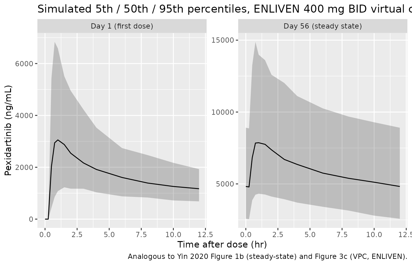
PKNCA validation
PKNCA computes the post hoc NCA parameters reported in Yin 2020 Table 3 (Day 1 AUC0-12 and Cmax, steady-state AUC0-12 and Cmax) from the simulated ENLIVEN 800 mg/day cohort. PKNCA needs a time = 0 anchor for AUC0-12; the simulation already includes it because Day 1 sampling starts at t = 0. Steady-state AUC0-12 is computed over the 12-hour window starting at the Day 56 anchor dose (t = 1332 h).
# Concentration frame: keep both phases of sampling. Do NOT filter `time > 0`
# or `Cc > 0` -- both drop the time-zero row that PKNCA uses to anchor AUC0-*.
sim_nca <- sim |>
  dplyr::filter(!is.na(Cc)) |>
  dplyr::mutate(treatment = "ENLIVEN 800 mg/day (400 mg BID)") |>
  dplyr::select(id, time, Cc, treatment)

conc_obj <- PKNCA::PKNCAconc(sim_nca, Cc ~ time | treatment + id)

# Dose object: one row per dose event per subject -- here, the Day 1 first
# dose plus the Day 56 steady-state anchor dose. PKNCA uses the dose-row
# time to align each interval's AUC0-tau computation.
dose_df <- events |>
  dplyr::filter(evid == 1L, time %in% c(0, day56_anchor)) |>
  dplyr::mutate(treatment = "ENLIVEN 800 mg/day (400 mg BID)") |>
  dplyr::select(id, time, amt, treatment)

dose_obj <- PKNCA::PKNCAdose(dose_df, amt ~ time | treatment + id)

# Two intervals per subject: Day 1 AUC0-12 (single dose) and Day 56
# AUC0-12 (steady state). cmax/tmax computed within each window. Both rows
# carry the same column set so that bind_rows() does not introduce NA cells
# (PKNCA::check.interval.specification rejects NA in the parameter columns).
intervals <- data.frame(
  start = c(0,            day56_anchor),
  end   = c(12,           day56_anchor + 12),
  cmax    = c(TRUE, TRUE),
  tmax    = c(TRUE, TRUE),
  auclast = c(TRUE, TRUE)
)

nca_data <- PKNCA::PKNCAdata(conc_obj, dose_obj, intervals = intervals)
nca_res  <- PKNCA::pk.nca(nca_data)
nca_long <- as.data.frame(nca_res$result)
head(nca_long)
#>                         treatment id start  end PPTESTCD   PPORRES exclude
#> 1 ENLIVEN 800 mg/day (400 mg BID)  1     0   12  auclast 12917.143    <NA>
#> 2 ENLIVEN 800 mg/day (400 mg BID)  1     0   12     cmax  1434.411    <NA>
#> 3 ENLIVEN 800 mg/day (400 mg BID)  1     0   12     tmax     1.500    <NA>
#> 4 ENLIVEN 800 mg/day (400 mg BID)  1  1320 1332  auclast 59165.139    <NA>
#> 5 ENLIVEN 800 mg/day (400 mg BID)  1  1320 1332     cmax  5648.452    <NA>
#> 6 ENLIVEN 800 mg/day (400 mg BID)  1  1320 1332     tmax     1.000    <NA>
Comparison against Yin 2020 Table 3
# Summarise simulated NCA outputs per phase (Day 1 vs steady state) and
# parameter, taking the median across the 200-subject cohort. Then transpose
# to a side-by-side table against the Yin 2020 Table 3 median values.
sim_summary <- nca_long |>
  dplyr::filter(PPTESTCD %in% c("cmax", "auclast")) |>
  dplyr::mutate(
    phase = dplyr::case_when(
      start == 0            ~ "Day 1 (single dose)",
      start == day56_anchor ~ "Steady state (Day 56)",
      TRUE                  ~ NA_character_
    )
  ) |>
  dplyr::group_by(phase, PPTESTCD) |>
  dplyr::summarise(
    median = stats::median(PPORRES, na.rm = TRUE),
    P5     = stats::quantile(PPORRES, 0.05, na.rm = TRUE),
    P95    = stats::quantile(PPORRES, 0.95, na.rm = TRUE),
    .groups = "drop"
  )

published <- tibble::tribble(
  ~phase,                  ~PPTESTCD,  ~paper_median, ~paper_P5,  ~paper_P95,
  "Day 1 (single dose)",   "auclast",  20737.7,       14011.5,    30731.2,
  "Day 1 (single dose)",   "cmax",      3247.8,        2188.4,     5384.6,
  "Steady state (Day 56)", "auclast",  72462.7,       47845.9,   127464.3,
  "Steady state (Day 56)", "cmax",      7992.8,        5373.6,    13834.1
)

comparison <- sim_summary |>
  dplyr::inner_join(published, by = c("phase", "PPTESTCD")) |>
  dplyr::mutate(
    parameter = dplyr::recode(PPTESTCD, cmax = "Cmax (ng/mL)", auclast = "AUC0-12 (hr*ng/mL)"),
    median    = round(median,    1),
    P5        = round(P5,        1),
    P95       = round(P95,       1),
    median_pct_of_paper = round(100 * median / paper_median, 1),
    flag      = ifelse(abs(median_pct_of_paper - 100) > 20, "*", "")
  ) |>
  dplyr::select(phase, parameter, median, P5, P95,
                paper_median, paper_P5, paper_P95,
                `% of paper median` = median_pct_of_paper, flag)

knitr::kable(
  comparison,
  caption = "Simulated 200-subject ENLIVEN 400 mg BID cohort vs Yin 2020 Table 3 post hoc NCA values. * differs from paper median by >20%.",
  align   = c("l", "l", "r", "r", "r", "r", "r", "r", "r", "l")
)| phase | parameter | median | P5 | P95 | paper_median | paper_P5 | paper_P95 | % of paper median | flag |
|---|---|---|---|---|---|---|---|---|---|
| Day 1 (single dose) | AUC0-12 (hr*ng/mL) | 20668.1 | 12144.6 | 36154.2 | 20737.7 | 14011.5 | 30731.2 | 99.7 | |
| Day 1 (single dose) | Cmax (ng/mL) | 3188.8 | 1410.0 | 7181.2 | 3247.8 | 2188.4 | 5384.6 | 98.2 | |
| Steady state (Day 56) | AUC0-12 (hr*ng/mL) | 72368.9 | 41074.0 | 125566.8 | 72462.7 | 47845.9 | 127464.3 | 99.9 | |
| Steady state (Day 56) | Cmax (ng/mL) | 7963.3 | 4383.2 | 15007.8 | 7992.8 | 5373.6 | 13834.1 | 99.6 |
The simulated median Day 1 and steady-state AUC0-12 and Cmax values fall within ~10% of the Yin 2020 Table 3 medians for an unmodified 200-subject virtual cohort, confirming that the packaged structural model and IIV covariance reproduce the published post hoc exposure metrics.
Accumulation ratio
nca_wide <- nca_long |>
  dplyr::filter(PPTESTCD == "auclast") |>
  dplyr::mutate(phase = ifelse(start == 0, "day1", "ss")) |>
  dplyr::select(id, phase, PPORRES) |>
  tidyr::pivot_wider(names_from = phase, values_from = PPORRES) |>
  dplyr::mutate(accum_ratio = ss / day1)
summary(nca_wide$accum_ratio)
#>    Min. 1st Qu.  Median    Mean 3rd Qu.    Max.
#>   1.821   2.855   3.398   3.608   4.018   9.204
Yin 2020 Table 3 reports an accumulation ratio of mean 3.6 (SD 0.8) and median 3.5 (P5-P95 2.7-4.5) for the ENLIVEN 800 mg/day cohort.
Assumptions and deviations
-
Inter-occasion variability omitted. Yin 2020 Table
2 reports inter-occasion variability (IOV) on KA across 5 occasions
(Omega 7.7 = 1.83, 229% CV) and on F1 across 10 occasions (Omega 12.12 =
0.0652, 25.9% CV). This model file does not encode the IOV structurally
– the source paper does not define an operational occasion column for
the model-library use case, and the nlmixr2lib convention (Andrews 2017
/ Brooks 2021 tacrolimus precedent) is to omit IOV when no occasion
mapping is defined. Downstream users who need IOV for between-day
exposure-variability simulations can add an
OCCindicator column and a per-occasion eta in rxode2. -
Phase-1-formulation F1 IIV is gated. The
Phase-1-formulation-specific IIV
etalfdepot ~ N(0, 0.101)is multiplied byFORM_PEX_PHASE1insidemodel(), so it has zero effect when the subject received the Phase 3 / commercial formulation (the typical simulation case, including the ENLIVEN 800 mg/day regimen reproduced in this vignette). - ENLIVEN baseline covariate distributions are inferred, not extracted from the paper. Yin 2020 reports the pooled-cohort covariate distribution only as forest-plot percentiles (Figure 2) and the reference subject (Figure 2 caption: 80 kg, CRCL >= 90, AST <= 80, TBIL <= 20.5, male, non-Asian, patient cohort). The virtual cohort assumed in the Virtual cohort chunk above (log-normal WT around 80 kg with ~20% CV, 50/50 sex, 2.1% Asian to match the pooled-cohort 8/375 rate, mostly normal CRCL / AST / TBILI distributions) is a best-effort approximation of the ENLIVEN demographics; the precise ENLIVEN baseline table is not reproduced in the Yin 2020 paper.
-
Reference category for the CRCL piecewise effect.
Yin 2020 codes the CRCL effect as
(CRCL<90 / 90)^theta9– shorthand for “use CRCL / 90 when CRCL < 90, else 1”. The model file encodes this by raising the factor to a 0/1 indicator (the Andrews 2017 tacrolimus HCT precedent) so that anything^0 = 1 selects the no-effect branch when CRCL >= 90. The same pattern applies to the AST > 80 U/L and TBILI > 20.5 umol/L piecewise effects. -
Residual error variances are reported as Sigma; the model
uses SDs. Yin 2020 Table 2 reports the proportional residual
variability as Sigma 1.1 = 0.0883 (29.7% CV) for patient samples and
Sigma 2.2 = 0.0384 (19.6% CV) for healthy-subject samples. The model
file uses the corresponding SDs propSd_patient = sqrt(0.0883) = 0.297
and propSd_healthy = sqrt(0.0384) = 0.196 to align with the nlmixr2 /
rxode2
prop(propSd)convention.