Gentamicin in plasma and saliva of neonates (Samb 2022)

Model and source

• Citation: Samb A, Kruizinga M, Tallahi Y, van Esdonk M, van Heel W, Driessen G, Bijleveld Y, Stuurman R, Cohen A, van Kaam A, de Haan TR, Mathot R. Saliva as a sampling matrix for therapeutic drug monitoring of gentamicin in neonates: A prospective population pharmacokinetic and simulation study. Br J Clin Pharmacol. 2022;88(4):1845-1855. doi:10.1111/bcp.15105. Plasma layer: Fuchs A, Guidi M, Giannoni E, et al. Population pharmacokinetic study of gentamicin in a large cohort of premature and term neonates. Br J Clin Pharmacol. 2014;78(5):1090-1101. doi:10.1111/bcp.12444.
• Description: Integrated plasma-saliva population PK model for intravenous gentamicin in preterm and term neonates (Samb 2022). Plasma is the Fuchs 2014 two-compartment neonatal model with every parameter held fixed (allometric weight scaling on CL/Q and Vc/Vp, linear centred effects of gestational age on CL and Vc, postnatal age on CL and concomitant dopamine on CL). A saliva compartment is appended as a driven, non-depleting hypothetical effect compartment: first-order transfer from central (kin_saliva = 0.023 1/h) and first-order loss from saliva (kel_saliva = 0.169 1/h), with the salivary concentration read on the central volume. Both saliva rate constants fall steeply with postmenstrual age (power exponents -8.8 and -5.1 referenced to 244.2 days), so gentamicin appears far more readily in the saliva of premature neonates. IIV on kel_saliva only (38% CV); log-scale (exponential) residual error on saliva (49.7%).
• Article: https://doi.org/10.1111/bcp.15105 (open access, PMC9298055)

Samb et al. measured gentamicin in saliva swabs from 54 preterm and term neonates and asked whether saliva could replace heel-lance plasma sampling for therapeutic drug monitoring (TDM). They kept plasma on the published Fuchs 2014 neonatal model with every parameter fixed (also packaged on its own as Fuchs_2014_gentamicin) and added one saliva compartment. That compartment is filled from central at rate kin_saliva (the paper’s k13) and emptied at rate kel_saliva (k30). It does not draw mass out of plasma. Postmenstrual age (PMA) has a strong negative effect on both saliva rate constants, so gentamicin reaches saliva far more readily in premature neonates.

Population

Fifty-four neonates were enrolled between October 2018 and March 2020 at the Emma Children’s Hospital (Amsterdam UMC) and the Juliana Children’s Hospital (The Hague); 60 had been planned, and the SARS-CoV-2 pandemic ended the study early. Table 1 of the paper gives the demographics: 57.4% male; gestational age (GA) median 34.8 weeks (range 24.3-41.7), with 21 neonates below 32 weeks, 13 at 32-37 weeks and 20 at or above 37 weeks; postnatal age (PNA) median 1.5 days (0.3-6.8); PMA median 244.2 days (170.5-294.2); current weight median 2.4 kg (0.7-4.3). Three neonates had perinatal asphyxia treated with controlled hypothermia. Each dose was a 0.5 h intravenous infusion: 5 mg/kg every 48 h (GA < 32 weeks), 5 mg/kg every 36 h (32-37 weeks), and 4 mg/kg every 24 h (Amsterdam) or 5 mg/kg every 36 h (The Hague) at or above 37 weeks.

Of 267 saliva swabs, 194 were analysed (73 had too little volume or were contaminated with blood), and 27 of the 194 were below the 0.056 mg/L LLOQ. The plasma data were 97 routine TDM concentrations.

The same information is available programmatically via rxode2::rxode(readModelDb("Samb_2022_gentamicin"))$population.

Source trace

Every ini() value carries an in-file comment naming its source. This table collects them in one place.

Equation / parameter	Value	Source location
lcl (CL, fixed)	0.089 L/h	Table S1 theta_CL (Fuchs 2014)
lvc (Vc, fixed)	0.908 L	Table S1 theta_Vc
lq (Q, fixed)	0.157 L/h	Table S1 theta_Q
lvp (Vp, fixed)	0.56 L	Table S1 theta_Vp
e_wt_cl_q, e_wt_vc_vp (fixed)	0.75, 1	Table S1 theta_CLWT / theta_QWT, theta_VcWT / theta_VpWT
e_ga_cl, e_ga_vc (fixed)	1.87, -0.922	Table S1 theta_CLGA, theta_VcGA
e_pna_cl (fixed)	0.054	Table S1 theta_CLPNA
e_conmed_dopa_cl (fixed)	-0.120	Table S1 theta_CLDOPA
IIV CL, IIV Vc, correlation (fixed)	28%, 18%, 87%	Table S1
addSd, propSd (fixed)	0.1 mg/L, 18%	Table S1 residual errors
Plasma covariate equations	(WT/2170 g)^theta * (1 + theta*(GA-34)/34) * (1 + theta*(PNA-1)/1) * (1 + theta*DOPA)	Table S1 TVCL / TVVC / Q / Vp equations
lkin_saliva (k13)	0.023 1/h	Table 2 final model (RSE 16%)
lkel_saliva (k30)	0.169 1/h	Table 2 final model (RSE 15%)
e_page_kin_saliva	-8.8	Table 2 theta_PMA_K13 (RSE 16%)
e_page_kel_saliva	-5.1	Table 2 theta_PMA_K30 (RSE 28%)
etalkel_saliva	38% CV -> 0.1349	Table 2 IIV k30
expSd_Csaliva	0.497	Table 2 sigma_prop (log-transformed data, Results 3.4)
Saliva covariate equations	k = theta * (PMA/244.2)^theta_PMA	Equation 1 and the equations printed under Table 2; 244.2 days = Table 1 median PMA
Saliva compartment structure	driven, no return	Methods 2.5 and Figure 1 (dashed central-to-saliva arrow)
Csaliva <- saliva / vc	–	Not printed; see Assumptions and deviations

Plasma layer is the packaged Fuchs 2014 model

Samb 2022 fixed every plasma parameter at the Fuchs 2014 estimates, and its saliva compartment does not deplete central. The typical-value plasma profile should therefore match Fuchs_2014_gentamicin to solver precision. Fuchs centres PNA by a ratio and Table S1 by a difference, but with a 1-day reference the two forms are the same.

mod <- readModelDb("Samb_2022_gentamicin")
mod_typ <- rxode2::zeroRe(mod)
#> ℹ parameter labels from comments will be replaced by 'label()'

# Representative neonates, one per GA group of Methods 2.2. The patients in
# Figure 3 are not identified beyond their GA group, so these covariates are
# illustrative: GA and PNA inside each band, with weight interpolated from the
# GA-weight pairs Fuchs 2014 uses for its own representative patients.
fuchs_ga <- c(26, 30, 34, 37, 40)
fuchs_bw <- c(0.890, 1.080, 2.120, 2.950, 3.580)
wt_for_ga <- function(ga) stats::approx(fuchs_ga, fuchs_bw, xout = ga, rule = 2)$y

reps <- tibble::tibble(
  id = 1:3,
  group = c("GA < 32 weeks", "GA 32-37 weeks", "GA >= 37 weeks"),
  GA = c(28, 34.8, 39),
  pna_days = c(2, 1.5, 2),
  # GA >= 37 weeks: the Hague regimen, 5 mg/kg every 36 h, which is the
  # interval visible in Figure 3C
  mg_per_kg = c(5, 5, 5),
  tau = c(48, 36, 36)
) |>
  mutate(
    WT = wt_for_ga(GA),
    PNA = pna_days / 30.4375,
    PAGE = (GA * 7 + pna_days) / 30.4375,
    CONMED_DOPA = 0
  )

make_rep_events <- function(r, n_dose, t_end, dt = 0.25) {
  amt <- r$mg_per_kg * r$WT
  doses <- tibble::tibble(
    time = (seq_len(n_dose) - 1) * r$tau, amt = amt, rate = amt / 0.5,
    evid = 1L, cmt = "central", dvid = NA_integer_
  )
  obs <- tibble::tibble(
    time = seq(0, t_end, by = dt), amt = NA_real_, rate = NA_real_,
    evid = 0L, cmt = "central", dvid = 1L
  )
  bind_rows(doses, obs) |>
    mutate(
      id = r$id, GA = r$GA, PNA = r$PNA, WT = r$WT, PAGE = r$PAGE,
      CONMED_DOPA = r$CONMED_DOPA, group = r$group
    ) |>
    arrange(time, desc(evid))
}

rep_events <- bind_rows(lapply(seq_len(nrow(reps)), function(i) {
  make_rep_events(reps[i, ], n_dose = 2, t_end = 2 * reps$tau[i])
}))

rep_sim <- rxode2::rxSolve(
  mod_typ,
  events = rep_events, keep = "group",
  useLinCmt = FALSE, atol = 1e-10, rtol = 1e-10
) |>
  as.data.frame()
#> ℹ omega/sigma items treated as zero: 'etalcl', 'etalvc', 'etalkel_saliva'
#> Warning: multi-subject simulation without without 'omega'

fuchs_sim <- rxode2::rxSolve(
  rxode2::zeroRe(readModelDb("Fuchs_2014_gentamicin")),
  events = rep_events |> select(-dvid),
  atol = 1e-10, rtol = 1e-10
) |>
  as.data.frame()
#> ℹ parameter labels from comments will be replaced by 'label()'
#> ℹ omega/sigma items treated as zero: 'etalcl', 'etalvc'
#> Warning: multi-subject simulation without without 'omega'

plasma_cmp <- inner_join(
  rep_sim |> select(id, time, Cc_samb = Cc),
  fuchs_sim |> select(id, time, Cc_fuchs = Cc),
  by = c("id", "time")
) |>
  filter(Cc_fuchs > 0)

max_rel <- max(abs(plasma_cmp$Cc_samb / plasma_cmp$Cc_fuchs - 1))
max_rel
#> [1] 2.406253e-11
# Same parameters and the same ODEs on both sides, so the only difference is
# solver error.
stopifnot(nrow(plasma_cmp) > 100, max_rel < 1e-6)

Replicate Figure 3: plasma and saliva in one neonate per GA group

Figure 3 of the paper shows individual fits for one neonate from each GA group. Below are the typical-value (population) profiles for the representative neonates defined above, over two dosing intervals.

rep_long <- rep_sim |>
  select(id, group, time, Cc, Csaliva) |>
  pivot_longer(c(Cc, Csaliva), names_to = "matrix", values_to = "conc") |>
  mutate(
    matrix = recode(matrix, Cc = "Plasma", Csaliva = "Saliva"),
    group = factor(group, levels = reps$group)
  ) |>
  filter(conc > 0)

ggplot(rep_long, aes(time, conc, linetype = matrix)) +
  geom_line() +
  scale_y_log10() +
  facet_wrap(~group, ncol = 1, scales = "free_x") +
  labs(
    x = "Time (h)", y = "Gentamicin (mg/L)", linetype = NULL,
    title = "Typical plasma and saliva gentamicin by GA group",
    caption = "Replicates the layout of Figure 3 of Samb 2022 (population predictions, representative covariates)."
  ) +
  theme_bw()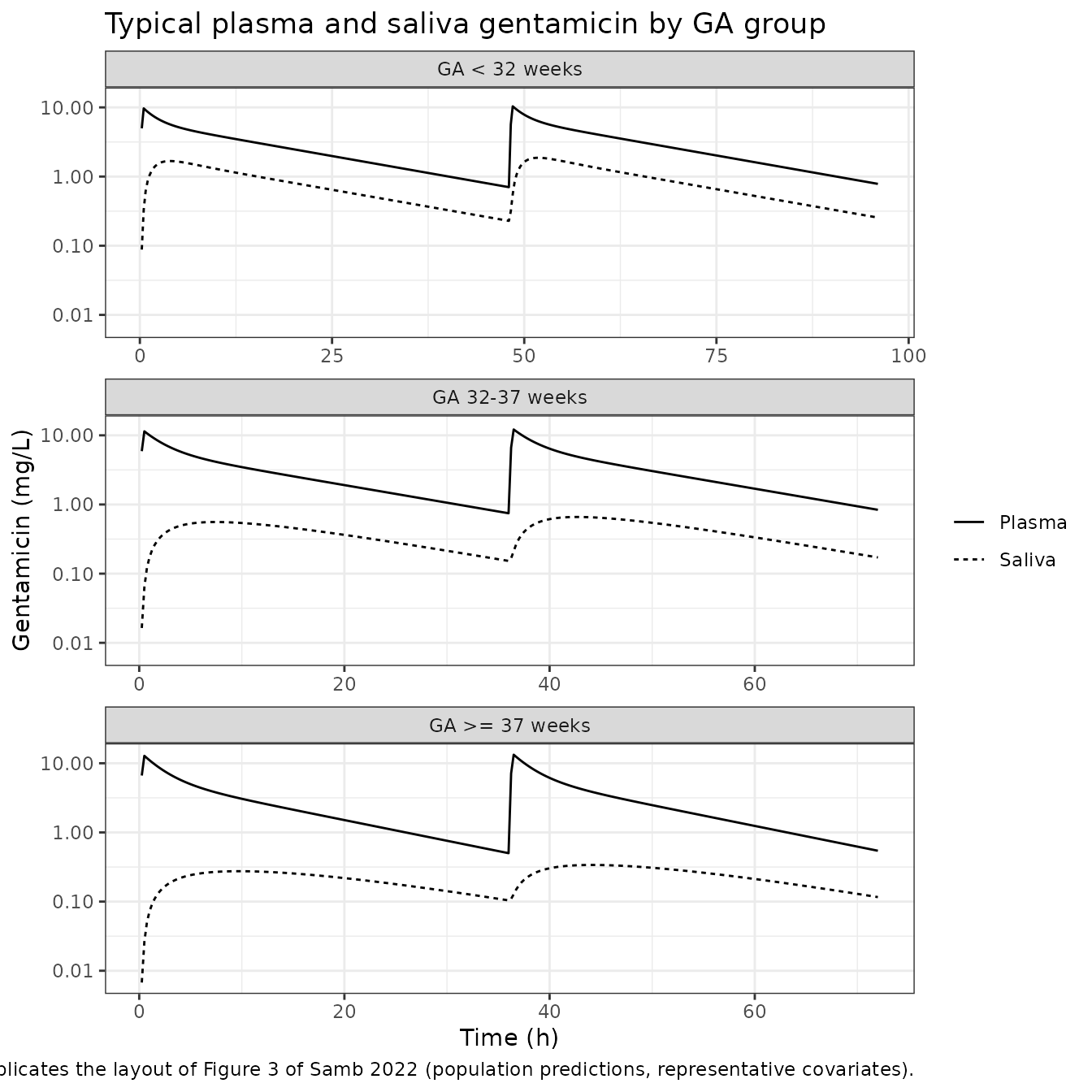

These are the levels read off Figure 3. They are approximate, because the plotted neonates’ exact covariates are not published:

fig3 <- tibble::tribble(
  ~group, ~quantity, ~figure3,
  "GA < 32 weeks", "Saliva peak, 1st interval (mg/L)", 2.6,
  "GA < 32 weeks", "Saliva/plasma ratio at end of 1st interval", 0.44,
  "GA 32-37 weeks", "Saliva peak, 1st interval (mg/L)", 0.47,
  "GA 32-37 weeks", "Saliva/plasma ratio at end of 1st interval", 0.22,
  "GA >= 37 weeks", "Saliva peak, 1st interval (mg/L)", 0.27,
  "GA >= 37 weeks", "Saliva/plasma ratio at end of 1st interval", 0.27
)

first_interval <- rep_sim |>
  left_join(reps |> select(id, tau), by = "id") |>
  filter(time <= tau)

model_fig3 <- first_interval |>
  group_by(group) |>
  summarise(
    peak = max(Csaliva),
    ratio_end = Csaliva[time == max(time)] / Cc[time == max(time)],
    .groups = "drop"
  ) |>
  pivot_longer(c(peak, ratio_end), names_to = "quantity", values_to = "model") |>
  mutate(quantity = recode(
    quantity,
    peak = "Saliva peak, 1st interval (mg/L)",
    ratio_end = "Saliva/plasma ratio at end of 1st interval"
  ))

fig3_cmp <- left_join(fig3, model_fig3, by = c("group", "quantity")) |>
  mutate(ratio_model_to_figure = model / figure3)

fig3_cmp |>
  mutate(across(c(model, ratio_model_to_figure), \(x) signif(x, 3))) |>
  rename(
    "GA group" = group, "Quantity" = quantity,
    "Figure 3 (read off)" = figure3, "Model" = model,
    "Model / figure" = ratio_model_to_figure
  ) |>
  knitr::kable(caption = "Representative typical-value profiles against levels read off Figure 3.")

Representative typical-value profiles against levels read off Figure 3.

GA group	Quantity	Figure 3 (read off)	Model	Model / figure
GA < 32 weeks	Saliva peak, 1st interval (mg/L)	2.60	1.680	0.645
GA < 32 weeks	Saliva/plasma ratio at end of 1st interval	0.44	0.325	0.740
GA 32-37 weeks	Saliva peak, 1st interval (mg/L)	0.47	0.558	1.190
GA 32-37 weeks	Saliva/plasma ratio at end of 1st interval	0.22	0.204	0.929
GA >= 37 weeks	Saliva peak, 1st interval (mg/L)	0.27	0.275	1.020
GA >= 37 weeks	Saliva/plasma ratio at end of 1st interval	0.27	0.208	0.769

# The figure shows individual fits of unidentified neonates, so the check is
# order-of-magnitude. Reading saliva on an implied 1 L volume instead of Vc
# would put the preterm saliva curve about threefold lower, and a wrong PMA
# exponent sign would invert the ordering across groups. Either fails here.
stopifnot(
  all(fig3_cmp$ratio_model_to_figure > 0.5),
  all(fig3_cmp$ratio_model_to_figure < 2)
)

The structure reproduces what Figure 3 shows. Saliva peaks within a few hours and closely follows plasma in the most premature neonate. In the term neonate it peaks late and stays flat.

Saliva:plasma ratio and postmenstrual age

The saliva compartment is driven by central and does not return drug to it. So once plasma is in its terminal phase (rate lambda_z), the saliva:plasma concentration ratio settles at kin_saliva / (kel_saliva - lambda_z), provided kel_saliva > lambda_z. Both rate constants fall with PMA, kin_saliva much faster (exponent -8.8 against -5.1). The ratio therefore drops steeply with maturity, which is the paper’s central finding.

# Single dose, solved long enough for every non-terminal exponential to vanish,
# then compared with the closed form built from the same typical parameters.
ratio_reps <- reps |> filter(GA < 37)  # kel_saliva well above lambda_z
long_events <- bind_rows(lapply(seq_len(nrow(ratio_reps)), function(i) {
  make_rep_events(ratio_reps[i, ], n_dose = 1, t_end = 150, dt = 5)
}))
long_sim <- rxode2::rxSolve(
  mod_typ,
  events = long_events, useLinCmt = FALSE, atol = 1e-14, rtol = 1e-12
) |>
  as.data.frame()
#> ℹ omega/sigma items treated as zero: 'etalcl', 'etalvc', 'etalkel_saliva'
#> Warning: multi-subject simulation without without 'omega'

analytic <- ratio_reps |>
  mutate(
    pma_days = PAGE * 30.4375,
    cl = 0.089 * (WT / 2.170)^0.75 * (1 + 1.87 * (GA - 34) / 34) *
      (1 + 0.054 * (pna_days - 1)),
    vc = 0.908 * (WT / 2.170) * (1 - 0.922 * (GA - 34) / 34),
    q = 0.157 * (WT / 2.170)^0.75,
    vp = 0.56 * (WT / 2.170),
    k10 = cl / vc, k12 = q / vc, k21 = q / vp,
    lambda_z = 0.5 * ((k10 + k12 + k21) - sqrt((k10 + k12 + k21)^2 - 4 * k10 * k21)),
    kin_saliva = 0.023 * (pma_days / 244.2)^-8.8,
    kel_saliva = 0.169 * (pma_days / 244.2)^-5.1,
    ratio_analytic = kin_saliva / (kel_saliva - lambda_z)
  )

ratio_cmp <- long_sim |>
  filter(time == 150) |>
  transmute(id, ratio_sim = Csaliva / Cc) |>
  inner_join(analytic |> select(id, group, lambda_z, kin_saliva, kel_saliva, ratio_analytic), by = "id")

ratio_cmp |>
  mutate(across(where(is.numeric) & !id, \(x) signif(x, 4))) |>
  select(group, lambda_z, kin_saliva, kel_saliva, ratio_analytic, ratio_sim) |>
  rename(
    "GA group" = group, "lambda_z (1/h)" = lambda_z,
    "kin_saliva (1/h)" = kin_saliva, "kel_saliva (1/h)" = kel_saliva,
    "Ratio, closed form" = ratio_analytic, "Ratio, simulated at 150 h" = ratio_sim
  ) |>
  knitr::kable(caption = "Terminal-phase saliva:plasma ratio, closed form against ODE solution.")

Terminal-phase saliva:plasma ratio, closed form against ODE solution.

GA group	lambda_z (1/h)	kin_saliva (1/h)	kel_saliva (1/h)	Ratio, closed form	Ratio, simulated at 150 h
GA < 32 weeks	0.04502	0.14560	0.4925	0.3254	0.3254
GA 32-37 weeks	0.05853	0.02227	0.1659	0.2075	0.2075

stopifnot(all(abs(ratio_cmp$ratio_sim / ratio_cmp$ratio_analytic - 1) < 1e-3))

pma_grid <- tibble::tibble(pma_days = seq(175, 290, by = 5)) |>
  mutate(
    kin_saliva = 0.023 * (pma_days / 244.2)^-8.8,
    kel_saliva = 0.169 * (pma_days / 244.2)^-5.1
  ) |>
  pivot_longer(-pma_days, names_to = "parameter", values_to = "value")

ggplot(pma_grid, aes(pma_days, value, linetype = parameter)) +
  geom_line() +
  geom_vline(xintercept = 244.2, colour = "grey60") +
  scale_y_log10() +
  labs(
    x = "Postmenstrual age (days)", y = "Typical rate constant (1/h)", linetype = NULL,
    caption = "Table 2 power equations; vertical line = reference PMA 244.2 days."
  ) +
  theme_bw()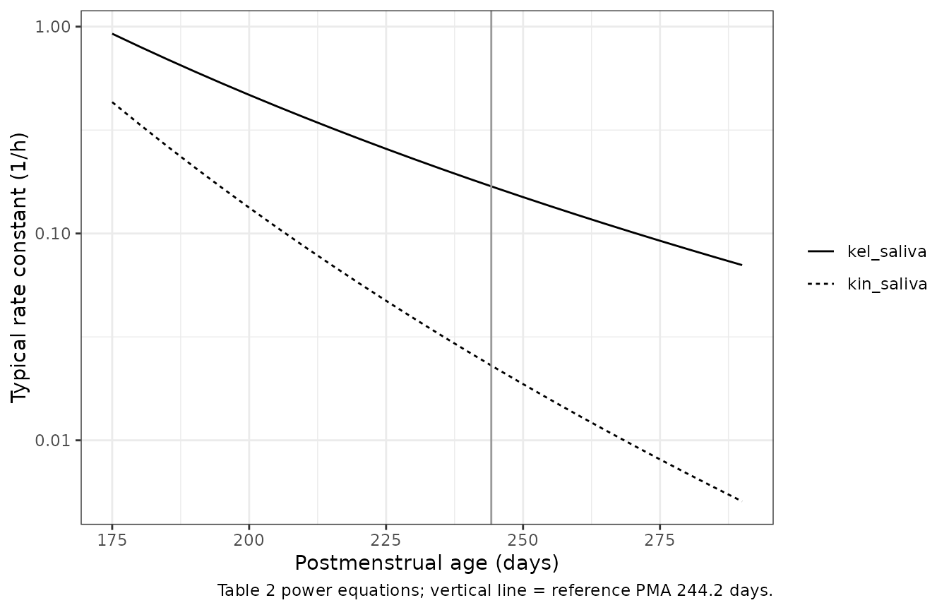

Virtual cohort and comparison with the Figure 4 pcVPC

The individual data are not public. The virtual cohort mirrors Table 1, with a few explicit assumptions. GA groups are sized in the Table 1 proportions (21:13:20, multiplied by three), and GA is uniform within each band over the observed 24.3-41.7 week range. PNA is log-uniform on 0.3-6.8 days, which gives a median near the observed 1.5 days. Weight is the GA-weight interpolation above with 10% log-normal scatter, and no neonate is on dopamine. Each neonate receives two doses of their group’s regimen (the Amsterdam regimen for GA >= 37 weeks).

set.seed(20220415)
rxode2::rxSetSeed(20220415)

n_grp <- c(63L, 39L, 60L)  # Table 1: 21 / 13 / 20 neonates, x3
cohort <- tibble::tibble(
  group = rep(c("GA < 32 weeks", "GA 32-37 weeks", "GA >= 37 weeks"), n_grp),
  GA = c(runif(n_grp[1], 24.3, 32), runif(n_grp[2], 32, 37), runif(n_grp[3], 37, 41.7)),
  mg_per_kg = rep(c(5, 5, 4), n_grp),
  tau = rep(c(48, 36, 24), n_grp)
) |>
  mutate(
    id = row_number(),
    pna_days = exp(runif(n(), log(0.3), log(6.8))),
    WT = wt_for_ga(GA) * exp(rnorm(n(), 0, 0.1)),
    PNA = pna_days / 30.4375,
    PAGE = (GA * 7 + pna_days) / 30.4375,
    CONMED_DOPA = 0
  )

summary(cohort |> select(GA, pna_days, WT) |> mutate(PMA_days = cohort$PAGE * 30.4375))
#>        GA           pna_days            WT            PMA_days    
#>  Min.   :24.30   Min.   :0.3036   Min.   :0.7487   Min.   :171.7  
#>  1st Qu.:29.42   1st Qu.:0.6084   1st Qu.:1.1005   1st Qu.:207.1  
#>  Median :34.31   Median :1.5173   Median :2.1516   Median :242.3  
#>  Mean   :33.84   Mean   :2.1182   Mean   :2.2233   Mean   :239.0  
#>  3rd Qu.:38.21   3rd Qu.:3.3083   3rd Qu.:3.2595   3rd Qu.:270.3  
#>  Max.   :41.53   Max.   :6.3292   Max.   :4.4357   Max.   :293.1

events <- bind_rows(lapply(seq_len(nrow(cohort)), function(i) {
  make_rep_events(cohort[i, ], n_dose = 2, t_end = 2 * cohort$tau[i], dt = 0.5)
}))

sim <- rxode2::rxSolve(
  mod,
  events = events, keep = c("group", "WT"),
  useLinCmt = FALSE
) |>
  as.data.frame() |>
  left_join(cohort |> select(id, tau), by = "id") |>
  mutate(
    tad = ifelse(time >= tau, time - tau, time),
    group = factor(group, levels = reps$group)
  )
#> ℹ parameter labels from comments will be replaced by 'label()'

stopifnot(!anyNA(sim$Cc), !anyNA(sim$Csaliva))

Figure 4 of the paper is a prediction-corrected VPC of the saliva data against time after the last dose. The medians below were read off its thick observed line. The simulated medians are individual predictions (IIV, no residual error). Prediction correction and the mixed sampling make the comparison approximate.

fig4_obs <- tibble::tribble(
  ~tad, ~median_obs,
  2.5, 0.70,
  7, 0.72,
  12, 0.42,
  18, 0.28,
  26, 0.33
)

sim_saliva <- sim |>
  filter(tad > 0, tad <= 36) |>
  mutate(bin = cut(tad, breaks = c(0, 5, 9.5, 15, 22, 30, 36))) |>
  group_by(bin) |>
  summarise(
    tad = median(tad),
    p10 = quantile(Csaliva, 0.1), p50 = median(Csaliva), p90 = quantile(Csaliva, 0.9),
    .groups = "drop"
  )

ggplot(sim_saliva, aes(tad)) +
  geom_ribbon(aes(ymin = p10, ymax = p90), fill = "grey85") +
  geom_line(aes(y = p50)) +
  geom_point(data = fig4_obs, aes(y = median_obs), shape = 21, size = 2.5) +
  scale_y_log10() +
  labs(
    x = "Time after dose (h)", y = "Saliva gentamicin (mg/L)",
    caption = "Line and band: simulated median and 10th-90th percentiles. Points: observed medians read off Figure 4 of Samb 2022."
  ) +
  theme_bw()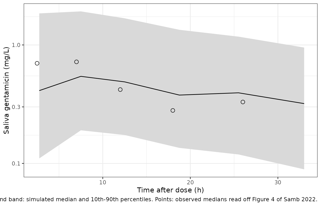

fig4_cmp <- fig4_obs |>
  mutate(sim_median = approx(sim_saliva$tad, sim_saliva$p50, xout = tad, rule = 2)$y) |>
  mutate(ratio = sim_median / median_obs)
knitr::kable(
  fig4_cmp |>
    mutate(across(c(sim_median, ratio), \(x) signif(x, 3))) |>
    rename(
      "Time after dose (h)" = tad, "Figure 4 observed median (mg/L)" = median_obs,
      "Simulated median (mg/L)" = sim_median, "Simulated / observed" = ratio
    ),
  caption = "Simulated saliva medians against the Figure 4 observed medians."
)

Simulated saliva medians against the Figure 4 observed medians.

Time after dose (h)	Figure 4 observed median (mg/L)	Simulated median (mg/L)	Simulated / observed
2.5	0.70	0.412	0.588
7.0	0.72	0.529	0.735
12.0	0.42	0.493	1.170
18.0	0.28	0.391	1.400
26.0	0.33	0.389	1.180

# Centre of the distribution, not its tails: a saliva volume or PMA exponent
# error shifts every bin severalfold.
stopifnot(abs(log(median(fig4_cmp$ratio))) < log(1.6), all(fig4_cmp$ratio > 0.4), all(fig4_cmp$ratio < 2.5))

PKNCA: first-dose exposure in plasma and saliva

The paper reports no NCA, so there is no published table to compare against. The first dosing interval is summarised per GA group for both matrices. The saliva:plasma AUC ratio gives the exposure-scale version of the PMA effect.

first <- sim |> filter(time <= tau)

nca_one <- function(df, conc_col) {
  conc <- df |>
    filter(!is.na(.data[[conc_col]])) |>
    transmute(id, group, time, conc = .data[[conc_col]])
  conc <- bind_rows(conc, conc |> distinct(id, group) |> mutate(time = 0, conc = 0)) |>
    distinct(id, group, time, .keep_all = TRUE) |>
    arrange(id, group, time)
  doses <- events |>
    filter(evid == 1L, time == 0) |>
    select(id, group, time, amt) |>
    mutate(group = factor(group, levels = reps$group))
  ints <- cohort |>
    distinct(group, tau) |>
    transmute(
      group = factor(group, levels = reps$group), start = 0, end = tau,
      cmax = TRUE, tmax = TRUE, auclast = TRUE
    )
  d <- PKNCA::PKNCAdata(
    PKNCA::PKNCAconc(conc, conc ~ time | group + id),
    PKNCA::PKNCAdose(doses, amt ~ time | group + id),
    intervals = ints
  )
  as.data.frame(PKNCA::pk.nca(d))
}

nca <- bind_rows(
  nca_one(first, "Cc") |> mutate(matrix = "Plasma"),
  nca_one(first, "Csaliva") |> mutate(matrix = "Saliva")
)

nca_summary <- nca |>
  filter(PPTESTCD %in% c("cmax", "tmax", "auclast")) |>
  group_by(matrix, group, PPTESTCD) |>
  summarise(median = signif(median(PPORRES), 3), .groups = "drop") |>
  pivot_wider(names_from = PPTESTCD, values_from = median)

nca_summary |>
  select(matrix, group, cmax, tmax, auclast) |>
  rename(
    "Matrix" = matrix, "GA group" = group, "Cmax (mg/L)" = cmax,
    "Tmax (h)" = tmax, "AUC0-tau (mg*h/L)" = auclast
  ) |>
  knitr::kable(caption = "Median first-dose NCA by matrix and GA group (simulated).")

Median first-dose NCA by matrix and GA group (simulated).

Matrix	GA group	Cmax (mg/L)	Tmax (h)	AUC0-tau (mg*h/L)
Plasma	GA < 32 weeks	9.880	0.50	125.0
Plasma	GA 32-37 weeks	11.600	0.50	102.0
Plasma	GA >= 37 weeks	10.200	0.50	65.5
Saliva	GA < 32 weeks	1.410	3.50	31.5
Saliva	GA 32-37 weeks	0.501	7.00	11.8
Saliva	GA >= 37 weeks	0.213	9.75	4.1

auc_ratio <- nca |>
  filter(PPTESTCD == "auclast") |>
  select(id, group, matrix, PPORRES) |>
  pivot_wider(names_from = matrix, values_from = PPORRES) |>
  mutate(sp_ratio = Saliva / Plasma) |>
  group_by(group) |>
  summarise(median_sp_auc_ratio = signif(median(sp_ratio), 3), .groups = "drop")

auc_ratio |>
  rename("GA group" = group, "Median saliva/plasma AUC0-tau" = median_sp_auc_ratio) |>
  knitr::kable(caption = "Saliva:plasma exposure ratio by GA group.")

Saliva:plasma exposure ratio by GA group.

GA group	Median saliva/plasma AUC0-tau
GA < 32 weeks	0.2590
GA 32-37 weeks	0.1170
GA >= 37 weeks	0.0612

# The plasma peak sits near the 8-12 mg/L clinical target band the paper
# quotes for standard dosing (Methods 2.6), and saliva exposure falls with
# maturity. Medians across 39-63 neonates per group, well clear of the bounds.
plasma_cmax <- nca_summary |> filter(matrix == "Plasma") |> pull(cmax)
stopifnot(
  all(plasma_cmax > 6), all(plasma_cmax < 16),
  auc_ratio$median_sp_auc_ratio[1] > 2 * auc_ratio$median_sp_auc_ratio[3]
)

Assumptions and deviations

• Saliva concentration is read on the central volume. Samb 2022 reports no saliva volume. Table 2 lists only k13, k30, the two PMA exponents, the residual error and the IIV, and the paper does not print the observation equation. Methods 2.5 calls the saliva compartment “similar to a hypothetical effect compartment model”, and the packaged model reads the saliva amount on Vc (Csaliva <- saliva / vc), as Nguyen_2026_linezolid does. The other reading, an implied 1 L scale (NONMEM’s default with no scale factor), is ruled out by Figure 3. It would leave the GA 32-37 week profile almost unchanged (Vc is about 1 L at 2.4 kg) but would put the saliva:plasma ratio of the most premature neonate at about 0.16. Figure 3A shows about 0.4, and the Vc reading gives about 0.33.
• Sign of the PMA exponents. The PDF typesetting drops the minus signs in Table 2. They are restored from the bootstrap columns (2.5th percentile -11.7 and -8.1, below the 97.5th percentiles -5.7 and -2.0) and from Results 3.4 (“a negative correlation between PMA and both the transport and elimination rate”). The Discussion quotes -5.5 for the k30 exponent, but Table 2 and Results 3.4 both give -5.1, which is used.
• IIV on k30 read as a CV. The paper does not say whether 38% is a CV or sqrt(omega^2) * 100, and its bootstrap percentile interval cannot tell the two apart. The packaged value is log(1 + 0.38^2) = 0.1349, the convention used for the same group’s Bijleveld_2017_gentamicin and for the plasma layer. The other reading gives 0.1444.
• Saliva residual error. “Logarithmic proportional error” on log-transformed data is an additive error on log(concentration), encoded as lnorm(expSd_Csaliva) with SD 0.497. The plasma residual error is the Fuchs 2014 combined additive + proportional model from Table S1, fixed. Samb 2022 also log-transformed the plasma data and does not say how this residual was carried on that scale. Saliva concentrations below the LLOQ were handled with the M3 method in estimation, which matters only for fitting.
• Postmenstrual age unit. The paper writes PMA in days. The canonical PAGE column is in months, and the model converts with PMA_days = PAGE * 30.4375. Supply PAGE consistent with GA and PNA (PMA in days = 7 * GA + PNA in days).
• Dopamine. The plasma layer keeps the Fuchs 2014 dopamine effect on CL. Samb 2022 does not report how many neonates received dopamine, and the virtual cohort assumes none did.
• Virtual cohort. The GA, PNA and weight distributions and the GA-to-weight interpolation (from Fuchs 2014’s representative GA-weight pairs) are assumptions. The paper’s own TDM simulation cohort (n = 3000, uniform GA) is shown only in a Supporting Information figure. Figure 3 and Figure 4 levels were read off the published figures by the maintainers.
• Not reproduced. The TDM target-attainment simulations (Figure 5) require Bayesian MAP re-estimation and a dose-adjustment rule. They are outside the scope of a model-library validation.