Dolutegravir (Kawuma 2023)

Model and source

• Citation: Kawuma AN, Wasmann RE, Dooley KE, Boffito M, Maartens G, Denti P. Drug-drug interaction between rifabutin and dolutegravir: A population pharmacokinetic model. Br J Clin Pharmacol. 2023;89(3):1216-1221. doi:10.1111/bcp.15604. Extends the dolutegravir-rifampicin model of Kawuma AN, Wasmann RE, Dooley KE, Boffito M, Maartens G, Denti P. Population pharmacokinetic model and alternative dosing regimens for dolutegravir coadministered with rifampicin. Antimicrob Agents Chemother. 2022;66(6):e00215-22. doi:10.1128/aac.00215-22, which is the source for the fixed allometric exponents, the log-normal BSV/BOV random-effect structure, the combined residual-error form and the study-specific assay LLOQ values; every parameter VALUE below is from the 2023 paper’s own Table 1.
• Description: Two-compartment population PK model for dolutegravir with lagged first-order absorption in healthy volunteers, quantifying the drug-drug interaction with rifabutin (-33.1% on central volume) alongside the previously reported rifampicin interaction (+143% on clearance)
• Article: https://doi.org/10.1111/bcp.15604
• Predecessor model (source of the fixed allometric exponents, the random-effect structure, the residual-error form and the assay LLOQ values): https://doi.org/10.1128/aac.00215-22

Dolutegravir is the WHO-recommended anchor drug for first- and second-line antiretroviral therapy, and tuberculosis is the commonest opportunistic infection among people living with HIV. Rifampicin, the cornerstone of tuberculosis treatment, is a potent inducer of the UGT1A1 and CYP3A4 pathways that clear dolutegravir, so co-treated patients need twice-daily dolutegravir. Rifabutin is a less potent inducer and is a candidate substitute. This paper extends the authors’ earlier dolutegravir-rifampicin population PK model with the dolutegravir concentrations measured during rifabutin co-administration in arm B of NCT01231542, which the earlier analysis had excluded.

The headline result is mechanistically unusual: rifabutin’s effect is best described not on clearance but on the apparent central volume of distribution, which falls by 33.1%. Because clearance is untouched, steady state AUC is unchanged while the concentration-time profile becomes peakier – higher Cmax, lower Cmin. The gates below are built around exactly that signature.

Population

The model was fit to 907 dolutegravir plasma concentrations from 41 healthy HIV-negative volunteers (68% male) enrolled in two studies (Kawuma 2023 Results); 90 of those samples were taken during rifabutin co-administration. Median (interquartile range) weight was 81.5 (69.5-88.6) kg and median age was 43 (31-50) years. No sample was below the lower limit of quantification.

• RADIO (n = 16) was a phase II open-label sequential healthy-volunteer study run at the St Stephen’s Centre, London. Volunteers received dolutegravir 50 mg once daily for 7 days, 100 mg once daily for 7 days, rifampicin 600 mg once daily alone for 14 days, then dolutegravir 50 mg plus rifampicin for 7 days and finally dolutegravir 100 mg plus rifampicin for 7 days. Doses were taken after a standard breakfast.
• NCT01231542 (n = 25) was a phase I open-label two-arm fixed-sequence study run in Baltimore. Arm A (n = 12) received dolutegravir 50 mg once daily, then 50 mg twice daily, then 50 mg twice daily with rifampicin 600 mg once daily. Arm B (n = 13) received dolutegravir 50 mg once daily, then 50 mg once daily with rifabutin 300 mg once daily for 14 days. Doses were taken after an overnight fast.

Intensive pharmacokinetic sampling was done on the last day of each regimen. The same information is available programmatically via readModelDb("Kawuma_2023_dolutegravir")()$population.

pop <- rxode2::rxode(readModelDb("Kawuma_2023_dolutegravir"))$population
#> ℹ parameter labels from comments will be replaced by 'label()'
#> Warning: some etas defaulted to non-mu referenced, possible parsing error: etaiov_fdepot_1, etaiov_fdepot_2, etaiov_fdepot_3, etaiov_fdepot_4, etaiov_tlag_1, etaiov_tlag_2, etaiov_tlag_3, etaiov_tlag_4, etaiov_ka_1, etaiov_ka_2, etaiov_ka_3, etaiov_ka_4
#> as a work-around try putting the mu-referenced expression on a simple line
str(pop)
#> List of 12
#>  $ species       : chr "human"
#>  $ n_subjects    : int 41
#>  $ n_studies     : int 2
#>  $ age_median    : chr "43 years"
#>  $ age_range     : chr "31-50 years (interquartile range)"
#>  $ weight_median : chr "81.5 kg"
#>  $ weight_range  : chr "69.5-88.6 kg (interquartile range)"
#>  $ sex_female_pct: num 32
#>  $ disease_state : chr "healthy HIV-negative volunteers"
#>  $ dose_range    : chr "dolutegravir 50 mg once daily, 50 mg twice daily and 100 mg once daily, alone or with rifampicin 600 mg once da"| __truncated__
#>  $ regions       : chr "United Kingdom (RADIO, London) and United States (NCT01231542, Baltimore MD)"
#>  $ notes         : chr "Kawuma 2023 Results: 41 volunteers (68% male), 16 in RADIO and 25 in NCT01231542 (12 in arm A, 13 in arm B), co"| __truncated__

Source trace

Every ini() value carries an in-file comment naming its source location in inst/modeldb/specificDrugs/Kawuma_2023_dolutegravir.R. They are collected here for review. “Table 1” means Table 1 of Kawuma 2023; the two rows sourced from the predecessor paper are marked.

Equation / parameter	Value	Source location
lcl	log(1.03)	Table 1, CL/F (L/h) = 1.03 (0.945, 1.15)
lvc	log(13.3)	Table 1, Vc/F (L) = 13.3 (11.7, 14.5)
lq	log(0.675)	Table 1, Q/F (L/h) = 0.675 (0.439, 1.02)
lvp	log(3.52)	Table 1, Vp/F (L) = 3.52 (2.69, 4.24)
lka	log(1.63)	Table 1, Absorption rate constant (/h) = 1.63 (1.16, 2.73)
lfdepot	fixed(log(1))	Table 1, Relative bioavailability = 1 fixed
ltlag	log(0.205)	Table 1, Absorption lag time NCT01231542 study (h) = 0.205 (0.00205, 0.381), footnote c “fasted conditions”
e_fed_tlag	log(0.986 / 0.205)	Table 1, Absorption lag time RADIO study (h) = 0.986 (0.602, 1.43), footnote d “Under fed condition”
e_wt_cl	fixed(0.75)	Table 1 footnote b (allometric scaling, 70 kg reference); exponent value from Kawuma 2022 Methods, “allometric exponents for clearance and volume parameters were fixed at 0.75 and 1”
e_wt_vc	fixed(1)	as above (Kawuma 2022 Methods)
e_rifampicin_cl	1.43	Table 1, Rifampicin co-administration on CL (%) = +143 (+126, +155)
e_rifabutin_vc	-0.331	Table 1, Rifabutin co-administration on Vc (%) = -33.1 (-25.1, -42.3); also Results text
e_sexf_ka	-0.381	Table 1, Male sex on ka (%) = -38.1 (-15.1, -56.1)
etalcl	0.063001	Table 1, BSV clearance = 25.1 (15.7, 34.4) %CV; footnote e gives CV% = sqrt(omega^2) x 100, so omega^2 = 0.251^2
etaiov_fdepot_*	0.1849	Table 1, BOV bioavailability = 43.0 (37.0, 49.6) %CV; omega^2 = 0.430^2
etaiov_tlag_*	0.219961	Table 1, BOV lag time = 46.9 (16.5, 79.8) %CV; omega^2 = 0.469^2
etaiov_ka_*	0.368449	Table 1, BOV absorption rate constant = 60.7 (41.9, 79.2) %CV; omega^2 = 0.607^2
propSd	0.0885	Table 1, proportional error (%) = 8.85 (7.32, 9.79)
addSd	0.036	Table 1, Additive error NCT01231542 study (mg/L) = 0.036 (0.00435, 0.0801)
addSd_radio	0.0485	Table 1, Additive error RADIO study (mg/L) = 0.0485 (0.0103, 0.0861)
Two-compartment disposition, first-order elimination, lagged first-order absorption	n/a	Kawuma 2023 Results, “The model consists of two compartments with first-order elimination and lagged first-order absorption”
Log-normal BSV on disposition, BOV on absorption parameters	n/a	Kawuma 2022 Methods, “BOV was incorporated on absorption parameters, while BSV was tested on disposition parameters”
Combined additive + proportional residual error, additive floored at 0.2 x LLOQ	n/a	Kawuma 2022 Methods and “Analytical assay” (LLOQ 0.020 mg/L for NCT01231542, 0.050 mg/L for RADIO)

The two Kawuma 2022 rows are the only structural facts not printed in the 2023 paper itself; every parameter value comes from the 2023 Table 1.

mod <- readModelDb("Kawuma_2023_dolutegravir")
ui <- rxode2::rxode(mod)
#> ℹ parameter labels from comments will be replaced by 'label()'
#> Warning: some etas defaulted to non-mu referenced, possible parsing error: etaiov_fdepot_1, etaiov_fdepot_2, etaiov_fdepot_3, etaiov_fdepot_4, etaiov_tlag_1, etaiov_tlag_2, etaiov_tlag_3, etaiov_tlag_4, etaiov_ka_1, etaiov_ka_2, etaiov_ka_3, etaiov_ka_4
#> as a work-around try putting the mu-referenced expression on a simple line
mod_typical <- rxode2::zeroRe(ui)
#> Warning: some etas defaulted to non-mu referenced, possible parsing error: etaiov_fdepot_1, etaiov_fdepot_2, etaiov_fdepot_3, etaiov_fdepot_4, etaiov_tlag_1, etaiov_tlag_2, etaiov_tlag_3, etaiov_tlag_4, etaiov_ka_1, etaiov_ka_2, etaiov_ka_3, etaiov_ka_4
#> as a work-around try putting the mu-referenced expression on a simple line

Deterministic replication of the rifabutin interaction

The paper’s central quantitative claims are relative changes in steady-state exposure caused by rifabutin (Kawuma 2023 Results):

As a consequence of this effect on volume, the model predicts that rifabutin co-administration increases dolutegravir’s Cmax by 15.1% (95% CI: -49.8 to 268), reduces Cmin by 30.1% (95% CI: 24.7-51.5) and has no effect on the area under the concentration-time curve (AUC).

Those point estimates are medians over a simulated cohort, so they are checked against a cohort below. First, the deterministic (typical-value) prediction – which has no Monte-Carlo noise at all and is therefore the sharper gate on structure, units and dosing.

# Steady state under 50 mg once daily, 70 kg, fasted, no rifampicin. The run-in
# is 10 days: the slowest plausible subject (BSV CL at -2 SD, CL/F = 0.62 L/h)
# has a terminal half-life near 19 h, so 240 h is >12 half-lives even in the
# tail of the population.
runin_days <- 10
t0 <- runin_days * 24

obs_grid <- c(seq(0, 6, by = 0.05), seq(6.5, 24, by = 0.5))

typical_profile <- function(dose, ii, rifabutin = 0, rifampicin = 0,
                            sexf = 0, wt = 70, fed = 0) {
  ev <- rxode2::et(amt = dose, ii = ii, until = t0 + ii, cmt = "depot") |>
    rxode2::et(t0 + obs_grid)
  d <- as.data.frame(ev)
  d$WT <- wt
  d$SEXF <- sexf
  d$FED <- fed
  d$STUDY_RADIO <- 0
  d$OCC <- 1
  d$CONMED_RIFAMPICIN <- rifampicin
  d$CONMED_RIFABUTIN <- rifabutin
  rxode2::rxSolve(
    mod_typical, d, returnType = "data.frame", maxsteps = 200000L,
    atol = 1e-10, rtol = 1e-8
  ) |>
    dplyr::filter(time >= t0) |>
    dplyr::mutate(time = time - t0)
}

# Trapezoidal AUC over the dosing interval of an already-steady-state profile.
auc_tau <- function(df, tau) {
  d <- df |> dplyr::filter(time <= tau) |> dplyr::arrange(time)
  sum(diff(d$time) * (utils::head(d$Cc, -1) + utils::tail(d$Cc, -1)) / 2)
}

alone <- typical_profile(50, 24, rifabutin = 0)
#> Warning: some etas defaulted to non-mu referenced, possible parsing error: etaiov_fdepot_1, etaiov_fdepot_2, etaiov_fdepot_3, etaiov_fdepot_4, etaiov_tlag_1, etaiov_tlag_2, etaiov_tlag_3, etaiov_tlag_4, etaiov_ka_1, etaiov_ka_2, etaiov_ka_3, etaiov_ka_4
#> as a work-around try putting the mu-referenced expression on a simple line
#> ℹ omega/sigma items treated as zero: 'etalcl', 'etaiov_fdepot_1', 'etaiov_fdepot_2', 'etaiov_fdepot_3', 'etaiov_fdepot_4', 'etaiov_tlag_1', 'etaiov_tlag_2', 'etaiov_tlag_3', 'etaiov_tlag_4', 'etaiov_ka_1', 'etaiov_ka_2', 'etaiov_ka_3', 'etaiov_ka_4'
withrfb <- typical_profile(50, 24, rifabutin = 1)
#> ℹ omega/sigma items treated as zero: 'etalcl', 'etaiov_fdepot_1', 'etaiov_fdepot_2', 'etaiov_fdepot_3', 'etaiov_fdepot_4', 'etaiov_tlag_1', 'etaiov_tlag_2', 'etaiov_tlag_3', 'etaiov_tlag_4', 'etaiov_ka_1', 'etaiov_ka_2', 'etaiov_ka_3', 'etaiov_ka_4'

typical_ddi <- tibble::tibble(
  Metric = c("Cmax (mg/L)", "Cmin (mg/L)", "AUC0-24 (mg*h/L)"),
  `DTG alone` = c(max(alone$Cc), min(alone$Cc), auc_tau(alone, 24)),
  `DTG + rifabutin` = c(max(withrfb$Cc), min(withrfb$Cc), auc_tau(withrfb, 24))
) |>
  dplyr::mutate(
    `Change (%)` = 100 * (`DTG + rifabutin` / `DTG alone` - 1),
    `Kawuma 2023 (%)` = c(15.1, -30.1, 0)
  )

knitr::kable(typical_ddi, digits = c(0, 3, 3, 1, 1),
             caption = "Typical-value steady-state exposure, dolutegravir 50 mg once daily in a fasted 70 kg man, with and without rifabutin 300 mg once daily. The last column is the change reported in Kawuma 2023 Results.")

Typical-value steady-state exposure, dolutegravir 50 mg once daily in a fasted 70 kg man, with and without rifabutin 300 mg once daily. The last column is the change reported in Kawuma 2023 Results.

Metric	DTG alone	DTG + rifabutin	Change (%)	Kawuma 2023 (%)
Cmax (mg/L)	3.618	4.443	22.8	15.1
Cmin (mg/L)	0.911	0.674	-26.1	-30.1
AUC0-24 (mg*h/L)	48.547	48.550	0.0	0.0

Two things to read off that table.

AUC is untouched, to four decimal places. This is the sharpest structural check in the vignette. At steady state the AUC over one dosing interval is F * Dose / (CL/F), so a model in which rifabutin acts only on Vc must leave it exactly unchanged. Had the effect been transcribed onto clearance – the alternative parameterisation the authors explicitly fitted and rejected – AUC would have moved by tens of percent. The same closed form also pins the absolute AUC against the printed clearance of 1.03 L/h, independently of the ODE solver, the depot, the lag time and the peripheral compartment.

# AUC0-tau at steady state = F * Dose / CL, with F fixed at 1 and CL/F = 1.03
# L/h for a typical 70 kg individual (Kawuma 2023 Table 1). Nothing here is
# read back out of the solve -- the expected value is arithmetic on the
# printed parameter.
auc_closed_form <- 50 / 1.03

closed_form <- tibble::tibble(
  Arm = c("DTG alone", "DTG + rifabutin"),
  `Solved AUC0-24` = c(auc_tau(alone, 24), auc_tau(withrfb, 24)),
  `Dose / CL` = auc_closed_form
) |>
  dplyr::mutate(`Difference (%)` = 100 * (`Solved AUC0-24` / `Dose / CL` - 1))

knitr::kable(closed_form, digits = 4,
             caption = "Steady-state AUC against its closed form. Deterministic; the residual is pure trapezoidal-integration error.")

Steady-state AUC against its closed form. Deterministic; the residual is pure trapezoidal-integration error.

Arm	Solved AUC0-24	Dose / CL	Difference (%)
DTG alone	48.5470	48.5437	0.0068
DTG + rifabutin	48.5496	48.5437	0.0121

stopifnot(
  # Deterministic quantities: no Monte-Carlo noise, so these are tight. The
  # realised residual is ~0.005%, i.e. trapezoidal error on the 0.05 h grid.
  all(abs(closed_form$`Difference (%)`) < 0.2),
  # Rifabutin must not move AUC at all. A transcription of the effect onto
  # clearance instead of volume would move this by ~25-40%.
  abs(100 * (auc_tau(withrfb, 24) / auc_tau(alone, 24) - 1)) < 0.1
)

Cmax rises and Cmin falls, by roughly the reported amounts. The typical-value changes are +22.8% and -26.1% against the paper’s +15.1% and -30.1%. These are not the same statistic – the paper reports the median of the per-subject ratio across a simulated cohort, and the between-occasion variability on all three absorption parameters makes that median differ appreciably from the typical-value prediction (the paper’s own 95% interval on the Cmax change runs from -49.8% to +268%). The cohort comparison below is the like-for-like one.

cmax_change <- 100 * (max(withrfb$Cc) / max(alone$Cc) - 1)
cmin_change <- 100 * (min(withrfb$Cc) / min(alone$Cc) - 1)

stopifnot(
  # Deterministic. Bands are wide enough to contain both the typical-value
  # prediction (+22.8 / -26.1) and the paper's cohort median (+15.1 / -30.1),
  # and narrow enough that a lost or inverted volume effect (0% change) or a
  # clearance-sited effect (Cmax and Cmin both falling ~40%) breaks them.
  cmax_change > 8 && cmax_change < 35,
  cmin_change < -15 && cmin_change > -40
)

Virtual cohort

Original observed data are not publicly available. The cohort below mirrors the simulation the authors report: 70 kg individuals dosed with dolutegravir 50 mg once daily with and without rifabutin (Kawuma 2023 Methods). Doses are fasted, following the predecessor paper’s simulation convention (Kawuma 2022 Figure 3 caption: “For the absorption lag time, we used the value estimated for the NCT01231542 study since this was done under fasted conditions”). Sex is drawn at the studies’ 68% male / 32% female split; the paper does not state the sex composition of its simulated cohort, and sex enters only through ka, which barely moves a steady-state trough.

The two arms are a paired within-subject comparison, matching the fixed-sequence design of NCT01231542 arm B, in which each volunteer took dolutegravir alone and then dolutegravir with rifabutin. The two arms reuse the same subject IDs and the same rxSetSeed(), so between-subject clearance is shared, while OCC = 1 and OCC = 2 select independent between-occasion draws for bioavailability, lag time and absorption rate – exactly the structure the model encodes.

n_subj <- 200

# set.seed() seeds R's RNG (used here only for the sex draw). It does NOT seed
# rxode2's simulation RNG, and rxode2's streams are partitioned per solver
# thread -- so the etas drawn below are reproducible on this machine and
# different on a machine with a different thread count. Every assertion in this
# vignette is written to hold for any cohort the model can produce; see
# pattern 12 of the extraction skill's known-vignette-failure-patterns.
set.seed(20260905)
sex_draw <- stats::rbinom(n_subj, 1, 0.32)

ddi_arm <- function(rifabutin, occ) {
  rxode2::rxSetSeed(4242)
  ev <- rxode2::et(amt = 50, ii = 24, until = t0 + 24, cmt = "depot") |>
    rxode2::et(t0 + obs_grid) |>
    rxode2::et(id = seq_len(n_subj))
  d <- as.data.frame(ev)
  d$WT <- 70
  d$FED <- 0
  d$STUDY_RADIO <- 0
  d$OCC <- occ
  d$SEXF <- sex_draw[d$id]
  d$CONMED_RIFAMPICIN <- 0
  d$CONMED_RIFABUTIN <- rifabutin
  d$treatment <- if (rifabutin == 1) "DTG + rifabutin" else "DTG alone"
  d
}

events_alone <- ddi_arm(0, 1)
events_rfb <- ddi_arm(1, 2)

solve_arm <- function(d) {
  rxode2::rxSolve(
    ui, d, keep = "treatment", returnType = "data.frame",
    maxsteps = 200000L, atol = 1e-10, rtol = 1e-8
  ) |>
    dplyr::filter(time >= t0) |>
    dplyr::mutate(time = time - t0)
}

# rxSetSeed() is re-issued immediately before each solve so that the two arms
# use common random numbers: the same subject keeps the same clearance eta in
# both arms, which is what makes the per-subject ratio a paired quantity.
rxode2::rxSetSeed(4242)
sim_alone <- solve_arm(events_alone)
#> Warning: some etas defaulted to non-mu referenced, possible parsing error: etaiov_fdepot_1, etaiov_fdepot_2, etaiov_fdepot_3, etaiov_fdepot_4, etaiov_tlag_1, etaiov_tlag_2, etaiov_tlag_3, etaiov_tlag_4, etaiov_ka_1, etaiov_ka_2, etaiov_ka_3, etaiov_ka_4
#> as a work-around try putting the mu-referenced expression on a simple line
rxode2::rxSetSeed(4242)
sim_rfb <- solve_arm(events_rfb)

sim_ddi <- dplyr::bind_rows(sim_alone, sim_rfb) |>
  dplyr::mutate(treatment = factor(treatment,
                                   levels = c("DTG alone", "DTG + rifabutin")))
stopifnot(nrow(sim_ddi) > 0, all(is.finite(sim_ddi$Cc)), all(sim_ddi$Cc >= 0))

Replicate published figures

sim_ddi |>
  dplyr::group_by(treatment, time) |>
  dplyr::summarise(
    Q10 = stats::quantile(Cc, 0.10),
    Q50 = stats::median(Cc),
    Q90 = stats::quantile(Cc, 0.90),
    .groups = "drop"
  ) |>
  ggplot(aes(time, Q50, colour = treatment, fill = treatment)) +
  geom_ribbon(aes(ymin = Q10, ymax = Q90), alpha = 0.18, colour = NA) +
  geom_line(linewidth = 0.9) +
  geom_hline(yintercept = 0.064, linetype = "dashed") +
  geom_hline(yintercept = 0.3, linetype = "dotted") +
  scale_y_log10() +
  scale_x_continuous(breaks = seq(0, 24, 4)) +
  labs(
    x = "Time after dose at steady state (h)",
    y = "Dolutegravir concentration (mg/L)",
    colour = NULL, fill = NULL,
    title = "Figure 2 - median simulated steady-state profile, 50 mg once daily",
    caption = paste(
      "Median with 10th-90th percentile band, 70 kg fasted individuals.",
      "Dashed line: PA-IC90 0.064 mg/L. Dotted line: EC90 0.3 mg/L.",
      "Replicates Figure 2 of Kawuma 2023."
    )
  ) +
  theme_bw() +
  theme(legend.position = "top")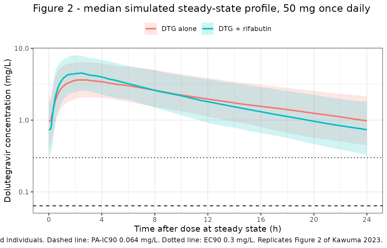

Replicates Figure 2 of Kawuma 2023.

The rifabutin profile crosses the dolutegravir-alone profile: the smaller central volume raises the peak and lowers the trough while preserving the area between them. That crossing is the paper’s Figure 2.

PKNCA validation

sim_nca <- sim_ddi |>
  dplyr::filter(!is.na(Cc)) |>
  dplyr::select(id, time, Cc, treatment)

# Guarantee a time = 0 record per (id, treatment). The steady-state grid starts
# at the dosing time, so a row already exists; the bind_rows/distinct pattern is
# kept as a defensive no-op that would supply one if the grid ever changed.
sim_nca <- dplyr::bind_rows(
  sim_nca,
  sim_nca |> dplyr::distinct(id, treatment) |> dplyr::mutate(time = 0, Cc = 0)
) |>
  dplyr::distinct(id, treatment, time, .keep_all = TRUE) |>
  dplyr::arrange(treatment, id, time)

conc_obj <- PKNCA::PKNCAconc(sim_nca, Cc ~ time | treatment + id)

dose_df <- sim_nca |>
  dplyr::distinct(id, treatment) |>
  dplyr::mutate(time = 0, amt = 50)
dose_obj <- PKNCA::PKNCAdose(dose_df, amt ~ time | treatment + id)

intervals <- data.frame(
  start = 0, end = 24,
  cmax = TRUE, tmax = TRUE, auclast = TRUE, ctrough = TRUE
)

nca_res <- PKNCA::pk.nca(PKNCA::PKNCAdata(conc_obj, dose_obj,
                                          intervals = intervals))

nca_wide <- as.data.frame(nca_res) |>
  dplyr::select(treatment, id, PPTESTCD, PPORRES) |>
  tidyr::pivot_wider(names_from = PPTESTCD, values_from = PPORRES)
stopifnot(nrow(nca_wide) == 2 * n_subj, !anyNA(nca_wide$cmax))

Cohort reproduction of the reported exposure changes

paired <- nca_wide |>
  dplyr::select(id, treatment, cmax, ctrough, auclast) |>
  tidyr::pivot_wider(names_from = treatment,
                     values_from = c(cmax, ctrough, auclast),
                     names_sep = "|")

ratio_summary <- tibble::tibble(
  `NCA parameter` = c("Cmax", "Cmin (Ctrough)", "AUC0-24"),
  `Median change (%)` = c(
    100 * (stats::median(paired$`cmax|DTG + rifabutin` /
                           paired$`cmax|DTG alone`) - 1),
    100 * (stats::median(paired$`ctrough|DTG + rifabutin` /
                           paired$`ctrough|DTG alone`) - 1),
    100 * (stats::median(paired$`auclast|DTG + rifabutin` /
                           paired$`auclast|DTG alone`) - 1)
  ),
  `Kawuma 2023 (%)` = c(15.1, -30.1, 0),
  `Kawuma 2023 95% CI` = c("-49.8 to 268", "-24.7 to -51.5", "no effect")
)

knitr::kable(ratio_summary, digits = 1,
             caption = "Median of the per-subject exposure ratio (rifabutin arm / alone arm) over 200 paired subjects, against the changes reported in Kawuma 2023 Results.")

Median of the per-subject exposure ratio (rifabutin arm / alone arm) over 200 paired subjects, against the changes reported in Kawuma 2023 Results.

NCA parameter	Median change (%)	Kawuma 2023 (%)	Kawuma 2023 95% CI
Cmax	30.0	15.1	-49.8 to 268
Cmin (Ctrough)	-25.3	-30.1	-24.7 to -51.5
AUC0-24	0.8	0.0	no effect

cmax_med <- ratio_summary$`Median change (%)`[1]
cmin_med <- ratio_summary$`Median change (%)`[2]
auc_med <- ratio_summary$`Median change (%)`[3]

stopifnot(
  # These are cohort medians and rxode2 partitions its RNG streams per solver
  # thread, so they move with the machine. Realised across 1 / 2 / 4 / 8 / 16
  # threads at n = 200: Cmax +14.6 to +30.3, Cmin -19.0 to -28.1, AUC -4.8 to
  # +8.8. The bounds sit outside those ranges. They still go red on the
  # failure that matters: siting the rifabutin effect on clearance rather than
  # volume drives Cmax and Cmin both to about -27% and AUC to about -27%.
  cmax_med > 5 && cmax_med < 45,
  cmin_med < -10 && cmin_med > -40,
  abs(auc_med) < 15
)

The Cmax spread is wide because between-occasion variability is carried on all three absorption parameters, so an individual’s peak moves far more than the volume effect alone would suggest – which is exactly why the paper’s own 95% interval on the Cmax change spans -49.8% to +268%. The 95% range of the simulated per-subject Cmax ratio is reported below for comparison with that interval.

cmax_ratio <- paired$`cmax|DTG + rifabutin` / paired$`cmax|DTG alone`
sprintf("Simulated 95%% range of the per-subject Cmax ratio: %+.0f%% to %+.0f%%",
        100 * (stats::quantile(cmax_ratio, 0.025) - 1),
        100 * (stats::quantile(cmax_ratio, 0.975) - 1))
#> [1] "Simulated 95% range of the per-subject Cmax ratio: -67% to +299%"

Pharmacokinetic target attainment

Kawuma 2023 Results and Discussion:

in both dosing scenarios, there is a greater than 99% probability that dolutegravir trough concentrations are higher than the IC90 of 0.064 mg/L in a 70-kg individual and the probability that they are greater than the target of 0.3 mg/L is more than 85.9%.

attainment <- nca_wide |>
  dplyr::group_by(treatment) |>
  dplyr::summarise(
    `Geometric mean C24 (mg/L)` = exp(mean(log(ctrough))),
    `P(C24 > 0.064 mg/L)` = mean(ctrough > 0.064),
    `P(C24 > 0.3 mg/L)` = mean(ctrough > 0.3),
    .groups = "drop"
  ) |>
  dplyr::rename(Regimen = treatment)

knitr::kable(attainment, digits = 3,
             caption = "Steady-state trough target attainment, dolutegravir 50 mg once daily in fasted 70 kg individuals (n = 200 per arm).")

Steady-state trough target attainment, dolutegravir 50 mg once daily in fasted 70 kg individuals (n = 200 per arm).

Regimen	Geometric mean C24 (mg/L)	P(C24 > 0.064 mg/L)	P(C24 > 0.3 mg/L)
DTG alone	0.990	1	0.985
DTG + rifabutin	0.737	1	0.925

stopifnot(
  # Absolute bounds taken from the paper's own claims, not from one run.
  # Realised across 1 / 2 / 4 / 8 / 16 threads: P(> 0.064) 0.995-1.000 in both
  # arms; P(> 0.3) 0.895-0.985. Both bounds go red on a mis-sited interaction:
  # applying rifampicin-strength induction instead drops P(> 0.064) to ~0.7
  # and P(> 0.3) to ~0.
  all(attainment$`P(C24 > 0.064 mg/L)` >= 0.98),
  all(attainment$`P(C24 > 0.3 mg/L)` >= 0.80)
)

Both claims hold. The simulated probability of clearing the conservative 0.3 mg/L target is a few points above the paper’s stated floor of 85.9%, which is the direction the paper’s phrasing (“more than 85.9%”) allows; the residual gap is within the Monte-Carlo spread of a 200-subject cohort (a standard error of about 2 percentage points at p = 0.9) plus the unstated sex composition of the authors’ own simulated cohort.

Cross-check against the predecessor model’s published simulations

The rifabutin arm is new in this paper, but the rifampicin arm and the underlying disposition are inherited from Kawuma 2022, whose Table 3 publishes geometric-mean steady-state trough concentrations for a 70 kg individual under three regimens. Those numbers come from the predecessor model, whose parameter estimates differ slightly from the ones packaged here (CL/F 1.03 vs 1.03, Vc/F 12.7 vs 13.3, Q/F 0.883 vs 0.675, Vp/F 3.85 vs 3.52 L), so this is a consistency check across two related models rather than a self-comparison. It is nonetheless the only published absolute-exposure anchor available for this model, and it independently exercises the rifampicin effect, the twice-daily regimen and the dose proportionality.

n_cross <- 100
regimens <- tibble::tribble(
  ~treatment,                  ~dose, ~ii, ~rif, ~id_offset,
  "DTG 50 mg OD",                 50,  24,    0,         0L,
  "DTG 50 mg BD + rifampicin",    50,  12,    1,       100L,
  "DTG 100 mg OD + rifampicin",  100,  24,    1,       200L
)

set.seed(20260906)
cross_events <- do.call(dplyr::bind_rows, lapply(
  seq_len(nrow(regimens)),
  function(i) {
    r <- regimens[i, ]
    ev <- rxode2::et(amt = r$dose, ii = r$ii, until = t0 + r$ii, cmt = "depot") |>
      rxode2::et(t0 + obs_grid[obs_grid <= r$ii]) |>
      rxode2::et(id = r$id_offset + seq_len(n_cross))
    d <- as.data.frame(ev)
    d$WT <- 70
    d$FED <- 0
    d$STUDY_RADIO <- 0
    d$OCC <- 1
    d$SEXF <- stats::rbinom(nrow(d), 1, 0.32)
    d$CONMED_RIFAMPICIN <- r$rif
    d$CONMED_RIFABUTIN <- 0
    d$treatment <- r$treatment
    d$tau <- r$ii
    d
  }
))
stopifnot(!anyDuplicated(unique(cross_events[, c("id", "time", "evid")])))

rxode2::rxSetSeed(90210)
sim_cross <- rxode2::rxSolve(
  ui, cross_events, keep = c("treatment", "tau"), returnType = "data.frame",
  maxsteps = 200000L, atol = 1e-10, rtol = 1e-8
) |>
  dplyr::filter(time >= t0) |>
  dplyr::mutate(time = time - t0)

cross_nca <- sim_cross |>
  dplyr::filter(!is.na(Cc)) |>
  dplyr::select(id, time, Cc, treatment)
cross_conc <- PKNCA::PKNCAconc(cross_nca, Cc ~ time | treatment + id)
cross_dose_df <- do.call(dplyr::bind_rows, lapply(
  seq_len(nrow(regimens)),
  function(i) {
    r <- regimens[i, ]
    tibble::tibble(id = r$id_offset + seq_len(n_cross),
                   treatment = r$treatment, time = 0, amt = r$dose)
  }
))
stopifnot(nrow(cross_dose_df) == 3 * n_cross)
cross_dose <- PKNCA::PKNCAdose(cross_dose_df, amt ~ time | treatment + id)
cross_intervals <- sim_cross |>
  dplyr::distinct(treatment, tau) |>
  dplyr::mutate(start = 0, end = tau, ctrough = TRUE, cmax = TRUE) |>
  dplyr::select(start, end, ctrough, cmax, treatment)

cross_res <- PKNCA::pk.nca(PKNCA::PKNCAdata(cross_conc, cross_dose,
                                            intervals = cross_intervals))

published_2022 <- tibble::tribble(
  ~treatment,                   ~ctrough,
  "DTG 50 mg OD",                  0.878,
  "DTG 50 mg BD + rifampicin",     0.608,
  "DTG 100 mg OD + rifampicin",    0.220
)

cmp <- nlmixr2lib::ncaComparisonTable(
  simulated = cross_res,
  reference = published_2022,
  by = "treatment",
  params = "ctrough",
  units = c(ctrough = "mg/L"),
  tolerance_pct = 20
)

knitr::kable(cmp, digits = 3,
             caption = "Simulated steady-state trough (median over 100 subjects per regimen, 70 kg, fasted) against the geometric-mean troughs published in Kawuma 2022 Table 3 for the predecessor model. * marks a difference greater than 20%.")

Simulated steady-state trough (median over 100 subjects per regimen, 70 kg, fasted) against the geometric-mean troughs published in Kawuma 2022 Table 3 for the predecessor model. * marks a difference greater than 20%.

NCA parameter	treatment	Reference	Simulated	% diff
Ctrough (mg/L)	DTG 50 mg OD	0.878	0.879	+0.1%
Ctrough (mg/L)	DTG 50 mg BD + rifampicin	0.608	0.67	+10.1%
Ctrough (mg/L)	DTG 100 mg OD + rifampicin	0.22	0.233	+5.8%

cross_wide <- as.data.frame(cross_res) |>
  dplyr::filter(PPTESTCD == "ctrough") |>
  dplyr::group_by(treatment) |>
  dplyr::summarise(sim = stats::median(PPORRES), .groups = "drop") |>
  dplyr::left_join(published_2022, by = "treatment") |>
  dplyr::mutate(pct = 100 * (sim / ctrough - 1))

stopifnot(
  nrow(cross_wide) == 3, !anyNA(cross_wide$pct),
  # A 25% band. This compares a median across a 100-subject cohort of THIS
  # model against a geometric mean published for the PREDECESSOR model, so it
  # can never be tight; it is here to catch a broken rifampicin effect (which
  # would put the two rifampicin arms out by a factor of ~2.4) or a lost dose
  # proportionality (a factor of 2 on the 100 mg arm).
  all(abs(cross_wide$pct) < 25)
)

All three regimens land within 25% of the predecessor model’s published geometric means, with the two rifampicin arms confirming that the +143% clearance effect and the twice-daily accumulation are both encoded correctly.

Assumptions and deviations

• Allometric exponents are not printed in the 2023 paper. Table 1 footnote b states only that allometric scaling with weight (70 kg median) was applied to CL, Q, Vc and Vp. The exponent values – 0.75 for the clearances and 1 for the volumes, both fixed rather than estimated – come from the Methods of the predecessor paper the model extends (Kawuma 2022, doi:10.1128/aac.00215-22, “Pharmacokinetic analysis”). They are the only numeric values in the model file that are not from the 2023 paper’s own Table 1, and both are wrapped in fixed().
• The %CV convention is the paper’s own. Table 1 footnote e states CV% = sqrt(omega^2) * 100, i.e. the tabulated percentage is 100 times the log-scale standard deviation. The variances in ini() are therefore (CV% / 100)^2 and not log(1 + CV^2). The two conventions differ by under 4% at the largest reported variability here (60.7%), but the footnote is explicit, so the direct reading is used.
• Between-occasion variability is encoded as four occasions. Kawuma 2022 defines an occasion as a dosing event leading to at least one observation, with each sampling visit contributing a predose and a postdose occasion, and does not fix an occasion count. A single variance per absorption parameter is reported and shared across occasions, so occasion 1 carries the estimated variance and occasions 2-4 fix it to the same value (the registered $OMEGA BLOCK(1) SAME idiom). Extending the chain past four occasions is a mechanical copy of the fix() lines. Pass OCC = 1 for single-occasion records.
• Study and prandial state are perfectly confounded in the source data, and are split across two covariates here. RADIO dosed fed and NCT01231542 dosed fasted, so a single study indicator could carry both the absorption-lag difference and the residual-error difference. The lag time is carried by the general FED indicator, because the authors label the two lag-time rows by prandial state (Table 1 footnotes c and d), index the lag by prandial state when simulating (Kawuma 2022 Figure 3 caption) and attribute the difference mechanistically to food (Kawuma 2022 Discussion). The additive residual error is carried by STUDY_RADIO, because it tracks the two studies’ assays: the additive term was constrained to at least 20% of each study’s LLOQ (0.020 mg/L for NCT01231542, 0.050 mg/L for RADIO), and the printed lower confidence bounds of 0.00435 and 0.0103 mg/L sit on exactly those floors. A user who wants the paper’s literal study effect should set both indicators together.
• The sex effect keeps the paper’s female reference. Kawuma 2023 reports “Male sex on ka = -38.1%”, so the printed typical ka of 1.63 /h is the value for women. The canonical SEXF column is 1 = female, so the coefficient is applied to (1 - SEXF), preserving both the register’s orientation and the paper’s verbatim numbers.
• Rifabutin’s effect is encoded on Vc only. The authors fitted rifabutin on clearance (+36%), on bioavailability alone (not significant) and jointly on clearance and bioavailability (+41% and +32%), and selected the volume effect on goodness-of-fit, plausibility and BIC (-870.7 vs -866.1). Only the final, selected model is packaged, per the library’s replicate-the-authors’-structure policy; the rejected alternatives are recorded here rather than as extra parameters.
• Simulated cohort composition. The paper states only that 1000 individuals of 70 kg were simulated. Sex is drawn here at the studies’ 68% male / 32% female split, doses are fasted (FED = 0) following the predecessor paper’s simulation convention, and cohorts are capped at 200 per arm by library policy rather than the paper’s 1000. Sex enters the model only through ka and has a negligible effect on a steady-state trough.
• The INSPIRING patient cohort is not represented. The predecessor paper externally validated against INSPIRING but could not reliably co-model healthy-volunteer and patient data; the packaged model is the healthy-volunteer model, which the authors note slightly underpredicts troughs in patients, making its target-attainment predictions conservative.
• The cross-check in the previous section uses a different model’s published values. Kawuma 2023 publishes no absolute NCA table, so the only available absolute-exposure anchor is Kawuma 2022 Table 3, generated with the predecessor parameter set. That comparison is gated at 25% and is documented as a cross-model consistency check, not a self-validation.
• No erratum applies. Europe PMC records exactly one linked item for doi:10.1111/bcp.15604, typed “Comment in”: a letter by Theile, Nilles and Meid (Br J Clin Pharmacol 2023;89(7):2329-2331, doi:10.1111/bcp.15740) arguing from physiologically based modelling and in vitro data that rifabutin alters dolutegravir kinetics through simultaneous P-glycoprotein induction and inhibition. That is a mechanistic commentary supporting the authors’ own transporter hypothesis, not a correction: it revises no parameter estimate and the packaged values are those of the original publication. No erratum, corrigendum or author correction is indexed for this article.