Zastaprazan (Yang 2024)
Source:vignettes/articles/Yang_2024_zastaprazan.Rmd
Yang_2024_zastaprazan.RmdModel and source
#> ℹ parameter labels from comments will be replaced by 'label()'Citation: Yang E, Hwang I, Ji SC, Kim J, Lee S. Population pharmacokinetic analysis of zastaprazan (JP-1366), a novel potassium-competitive acid blocker, in patients and healthy volunteers. CPT Pharmacometrics Syst Pharmacol. 2024;13(12):2150-2158. doi:10.1002/psp4.13228.
Description: Two-compartment population PK model with Erlang-type absorption through six sequential first-order transit steps and first-order elimination for zastaprazan (JP-1366), a potassium-competitive acid blocker, after oral dosing in patients with erosive gastroesophageal reflux disease (GERD) and in healthy volunteers (Yang 2024). Pooled analysis of 1590 plasma concentrations from 160 subjects across one phase 1 study in healthy volunteers (intensive sampling) and one phase 2 study in patients with erosive GERD (trough sampling), fit in NONMEM 7.4.4 by FOCEI. All six absorption steps share a single transit rate constant Ktr, so the absorption-time distribution is Erlang with shape 6 and rate Ktr. Disease status is the only retained covariate: apparent clearance is 41.4% lower in patients with GERD than in healthy volunteers, via the linear form CL/F = 29.4 * (1 - 0.414 * DIS_GERD). Typical values are for a healthy volunteer. Inter-individual variability is log-normal on Ktr, CL/F, Vc/F and Vp/F (none on Q/F); residual variability is proportional. CYP2C19 phenotype had no meaningful effect on zastaprazan PK, consistent with CYP3A-mediated rather than CYP2C19-mediated metabolism.
Article: https://doi.org/10.1002/psp4.13228
Zastaprazan (JP-1366) is a potassium-competitive acid blocker (P-CAB) approved in the Republic of Korea for erosive gastroesophageal reflux disease (GERD) at 20 mg once daily. Yang 2024 pooled a phase 1 study in healthy volunteers with intensive sampling and a phase 2 study in patients with erosive GERD with sparse trough sampling, and described the plasma PK with a two-compartment model, Erlang-type absorption through six sequential first-order steps, and first-order elimination.
Population
The analysis dataset comprised 1590 plasma concentrations from 160 subjects: 92 patients with erosive GERD contributing 95 (trough) observations and 68 healthy volunteers contributing 1495 (intensively sampled) observations (Yang 2024 Results, “Study population”). Median age was 39 years (range 19-74) and median body weight 71.0 kg (range 43.4-106.2); 129 of 160 subjects (80.6%) were male (Yang 2024 Table 1). The two cohorts differ substantially in age (patients median 58 years versus healthy volunteers median 28 years) and in sex balance (the healthy cohort was 100% male), so age and sex are partly confounded with disease status in this dataset.
CYP2C19 phenotype was determined for 156 of the 160 subjects (70 normal, 69 intermediate, 17 poor metabolizers) and had no meaningful effect on zastaprazan PK, consistent with metabolism by CYP3A4/CYP3A5 rather than CYP2C19. Eleven of the 92 patients (12.0%) were Helicobacter pylori positive; exposure in those patients fell within the range of the H. pylori-negative patients (Yang 2024 Figure S2).
Doses were oral: single 5-60 mg or once-daily 5-40 mg for 7 days in the healthy volunteers (Study 1), and once-daily 10-40 mg for 4 or 8 weeks in the patients (Study 2).
The same information is available programmatically from the model’s
population metadata:
str(ui$population, vec.len = 2)
#> List of 15
#>  $ species       : chr "human"
#>  $ n_subjects    : int 160
#>  $ n_studies     : int 2
#>  $ n_observations: int 1590
#>  $ age_range     : chr "Total 19-74 years (median 39); patients with erosive GERD 24-74 years (median 58); healthy volunteers 19-45 years (median 28)"
#>  $ age_median    : chr "39 years"
#>  $ weight_range  : chr "Total 43.4-106.2 kg (median 71.0); patients with erosive GERD 43.4-106.2 kg (median 69.7); healthy volunteers 5"| __truncated__
#>  $ weight_median : chr "71.0 kg"
#>  $ sex_female_pct: num 19.4
#>  $ race_ethnicity: chr "Not reported; Yang 2024 Table 1 tabulates no race or ethnicity"
#>  $ disease_state : chr "92 patients with erosive gastroesophageal reflux disease (phase 2 Study 2) and 68 healthy volunteers without an"| __truncated__
#>  $ dose_range    : chr "Study 1 (healthy volunteers): oral single doses of 5-60 mg or once-daily multiple doses of 5-40 mg for 7 consec"| __truncated__
#>  $ regions       : chr "Not explicitly stated; both studies were run by investigators at Seoul National University College of Medicine "| __truncated__
#>  $ genotype      : chr "CYP2C19 phenotype identified for 156 of 160 subjects: 70 normal metabolizers (*1/*1, 43.8%), 69 intermediate me"| __truncated__
#>  $ notes         : chr "Demographics from Yang 2024 Table 1 (median and range for age and weight, n (%) for categorical variables); stu"| __truncated__
Source trace
Every ini() entry carries an in-file comment naming its
source location in
inst/modeldb/specificDrugs/Yang_2024_zastaprazan.R. They
are collected here for review. All values are the final
model column of Yang 2024 Table 2; the base-model column and
the bootstrap medians are recorded in the in-file comments only.
| Equation / parameter | Value | Source location |
|---|---|---|
lktr (Ktr) |
13.6 1/h | Table 2, final model (RSE 3.9%) |
lcl (CL/F, healthy volunteer) |
29.4 L/h | Table 2, final model (RSE 5.1%) |
e_dis_gerd_cl (disease-status effect on CL/F) |
-0.414 | Table 2 “Effect of disease status” (RSE 8.6%) |
lvc (Vc/F) |
97.3 L | Table 2, final model (RSE 5.0%) |
lq (Q/F) |
29.1 L/h | Table 2, final model (RSE 6.7%) |
lvp (Vp/F) |
148.0 L | Table 2, final model (RSE 4.6%) |
etalktr |
26.1 %CV -> log(1 + 0.261^2)
|
Table 2 “IIV Ktr (CV%)” (RSE 17.8%) |
etalcl |
38.2 %CV -> log(1 + 0.382^2)
|
Table 2 “IIV CL/F (CV%)” (RSE 6.7%) |
etalvc |
27.4 %CV -> log(1 + 0.274^2)
|
Table 2 “IIV Vc/F (CV%)” (RSE 13.8%) |
etalvp |
28.0 %CV -> log(1 + 0.280^2)
|
Table 2 “IIV Vp/F (CV%)” (RSE 10.3%) |
| no IIV on Q/F | n/a | Results: “The final model included the IIV for most PK parameters except for Q/F” |
propSd |
0.349 | Table 2 “Proportional residual error (%)” = 34.9% (RSE 3.6%) |
| Erlang absorption: 6 sequential Ktr steps | n/a | Figure 1 (six boxes, five inter-box Ktr arrows plus a sixth Ktr arrow into the central compartment); Results: “transit through six sequential compartments under Erlang-type model” |
CL/F = 29.4 * (1 - 0.414 * DIS_GERD) |
n/a | Table 2 footnote a: “CL/F (L/h) = 29.4 x (1-0.414 x PT); PT = 1 (patient) or 0 (healthy volunteer)” |
| Two-compartment distribution, first-order elimination | n/a | Figure 1 and Results, “Final population pharmacokinetic model” |
| Proportional residual error only | n/a | Results: “the residual variability was described by proportional error model” |
The model encodes the absorption chain as depot (Figure
1 box 1) followed by transit1-transit5 (boxes
2-6), so the dose passes through exactly six first-order transfers all
governed by the single estimated Ktr. That is an Erlang
absorption-time distribution with shape 6 and rate Ktr,
mean absorption time 6 / 13.6 = 0.44 h.
Virtual cohort
Original observed data are not publicly available. The cohort below reproduces the Monte Carlo design of Yang 2024’s “Model-based simulation” section: once-daily oral doses of 10, 20 or 40 mg for 4 weeks, in patients with GERD and in healthy volunteers. The paper simulated 1000 subjects per arm; this vignette uses 200 per arm, which is ample for the median and percentile comparisons below.
Disease status is the model’s only covariate, so no other covariate distribution needs to be constructed.
set.seed(20241213)

n_per_arm  <- 200L
tau        <- 24      # dosing interval (h)
n_doses    <- 28L     # 4 weeks of once-daily dosing
t_last     <- (n_doses - 1L) * tau   # time of the final dose, 648 h

# Observation grid: daily troughs to show the approach to steady state, plus a
# dense grid across the final (steady-state) dosing interval. `cmt` is the ODE
# state `central`; rxode2 returns the algebraic observable Cc at those rows.
obs_troughs <- seq(tau, t_last - tau, by = tau)
obs_ss      <- t_last + seq(0, tau, by = 0.25)

make_cohort <- function(n, dose, dis_gerd, id_offset = 0L) {
  arm <- paste0(dose, " mg ", if (dis_gerd == 1L) "GERD" else "healthy")
  doses <- tidyr::expand_grid(
    id   = id_offset + seq_len(n),
    time = seq(0, t_last, by = tau)
  ) |>
    dplyr::mutate(amt = dose, evid = 1L, cmt = "depot")
  obs <- tidyr::expand_grid(
    id   = id_offset + seq_len(n),
    time = c(obs_troughs, obs_ss)
  ) |>
    dplyr::mutate(amt = NA_real_, evid = 0L, cmt = "central")
  dplyr::bind_rows(doses, obs) |>
    dplyr::mutate(DIS_GERD = dis_gerd, arm = arm, dose_mg = dose) |>
    dplyr::arrange(id, time, dplyr::desc(evid))
}

arms <- tidyr::expand_grid(dose = c(10, 20, 40), dis_gerd = c(1L, 0L)) |>
  dplyr::mutate(id_offset = (dplyr::row_number() - 1L) * n_per_arm)

events <- do.call(
  dplyr::bind_rows,
  Map(make_cohort,
      n         = n_per_arm,
      dose      = arms$dose,
      dis_gerd  = arms$dis_gerd,
      id_offset = arms$id_offset)
)

# Disjoint IDs across arms are mandatory: rxSolve keys subjects on `id`, and a
# collision silently merges two arms into one subject receiving the summed dose.
stopifnot(!anyDuplicated(unique(events[, c("id", "time", "evid")])))
stopifnot(dplyr::n_distinct(events$id) == nrow(arms) * n_per_arm)
Simulation
Cc in the rxode2 output is the individual prediction
(IPRED, free of residual error); sim additionally carries
the proportional residual error. Both are used below, for different
comparisons.
mod <- readModelDb("Yang_2024_zastaprazan")

sim <- rxode2::rxSolve(
  mod, events = events,
  keep = c("arm", "dose_mg", "DIS_GERD")
) |>
  as.data.frame()
#> ℹ parameter labels from comments will be replaced by 'label()'

sim_ss <- sim |>
  dplyr::filter(!is.na(Cc), time >= t_last) |>
  dplyr::mutate(tad = time - t_last)
Replicate published figures
# Replicates Figure 4 of Yang 2024: simulated steady-state profiles over one
# dosing interval after 10, 20 or 40 mg once daily, GERD patients vs healthy
# volunteers. Median with 5th-95th percentile ribbon, matching the paper's
# figure legend.
sim_ss |>
  dplyr::mutate(cohort = ifelse(DIS_GERD == 1, "GERD patients", "Healthy volunteers"),
                dose_lab = factor(paste0(dose_mg, " mg"),
                                  levels = c("10 mg", "20 mg", "40 mg"))) |>
  dplyr::group_by(dose_lab, cohort, tad) |>
  dplyr::summarise(
    Q05 = quantile(Cc, 0.05),
    Q50 = median(Cc),
    Q95 = quantile(Cc, 0.95),
    .groups = "drop"
  ) |>
  ggplot(aes(tad, Q50, colour = cohort, fill = cohort)) +
  geom_ribbon(aes(ymin = Q05, ymax = Q95), alpha = 0.2, colour = NA) +
  geom_line(linewidth = 0.7) +
  facet_wrap(~dose_lab) +
  labs(x = "Time after dose (h)", y = "Zastaprazan concentration (ug/L)",
       colour = NULL, fill = NULL,
       title = "Figure 4 - simulated steady-state profiles",
       caption = "Replicates Figure 4 of Yang 2024.") +
  theme(legend.position = "bottom")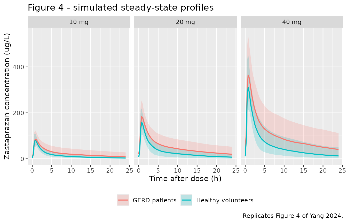
# Replicates Figure 5 of Yang 2024: distributions of steady-state Cmax and
# AUCtau by dose and cohort. AUCtau is the linear-trapezoid integral of the
# individual prediction over the final dosing interval.
per_subject <- sim_ss |>
  dplyr::arrange(id, tad) |>
  dplyr::group_by(id, arm, dose_mg, DIS_GERD) |>
  dplyr::summarise(
    cmax_ss = max(Cc),
    tmax_ss = tad[which.max(Cc)],
    auctau  = sum(diff(tad) * (head(Cc, -1) + tail(Cc, -1)) / 2),
    .groups = "drop"
  ) |>
  dplyr::mutate(cohort = ifelse(DIS_GERD == 1, "GERD patients", "Healthy volunteers"),
                dose_lab = factor(paste0(dose_mg, " mg"),
                                  levels = c("10 mg", "20 mg", "40 mg")))

per_subject |>
  tidyr::pivot_longer(c(cmax_ss, auctau), names_to = "metric", values_to = "value") |>
  dplyr::mutate(metric = ifelse(metric == "cmax_ss",
                                "Cmax,ss (ug/L)", "AUCtau (h*ug/L)")) |>
  ggplot(aes(dose_lab, value, fill = cohort)) +
  geom_boxplot(outlier.size = 0.4) +
  facet_wrap(~metric, scales = "free_y") +
  labs(x = NULL, y = NULL, fill = NULL,
       title = "Figure 5 - steady-state exposure by dose and cohort",
       caption = "Replicates Figure 5 of Yang 2024.") +
  theme(legend.position = "bottom")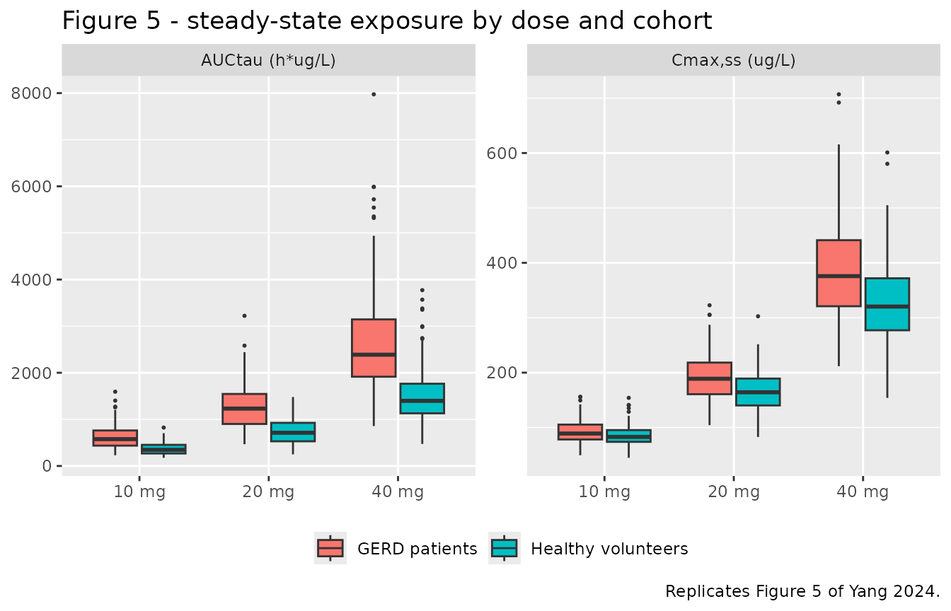
Closed-form and analytic checks
Three checks do not depend on the simulation grid at all and are therefore the sharpest gates available for this model.
1. Steady-state AUCtau must equal Dose / (CL/F) exactly. With a linear model and complete dosing intervals this is an identity, so any deviation would signal a structural transcription error rather than a numerical tolerance.
2. Analytic terminal half-life. The terminal rate
constant is the smaller root of the two-compartment characteristic
equation, computed from the typical parameters directly rather than by
regression on a simulated grid (a windowed regression or PKNCA’s
lambda.z can disagree with the analytic value by 20% or
more when the sampling window is not deep in the terminal phase).
3. Disease-status contrasts. Because the disease
effect enters CL/F only, the typical AUCtau ratio is exactly
1 / (1 - 0.414).
theta   <- ui$theta
cl_hv   <- exp(theta[["lcl"]])
cl_gerd <- cl_hv * (1 + theta[["e_dis_gerd_cl"]])
vc      <- exp(theta[["lvc"]])
q       <- exp(theta[["lq"]])
vp      <- exp(theta[["lvp"]])

terminal_thalf <- function(cl) {
  kel <- cl / vc; k12 <- q / vc; k21 <- q / vp
  s <- kel + k12 + k21
  beta <- (s - sqrt(s^2 - 4 * kel * k21)) / 2
  log(2) / beta
}

typical_auc <- per_subject |>
  dplyr::group_by(dose_lab, cohort, dose_mg, DIS_GERD) |>
  dplyr::summarise(auctau_median = median(auctau), .groups = "drop") |>
  dplyr::mutate(dose_over_cl = dose_mg / ifelse(DIS_GERD == 1, cl_gerd, cl_hv) * 1000,
                pct_diff = 100 * (auctau_median - dose_over_cl) / dose_over_cl)

typical_auc |>
  dplyr::select(dose_lab, cohort, auctau_median, dose_over_cl, pct_diff) |>
  dplyr::rename(
    "Dose"                       = dose_lab,
    "Cohort"                     = cohort,
    "Simulated median AUCtau"    = auctau_median,
    "Dose / (CL/F)"              = dose_over_cl,
    "% difference"               = pct_diff
  ) |>
  knitr::kable(
    digits  = 1,
    caption = "Steady-state AUCtau (h*ug/L) against the closed-form identity Dose / (CL/F)."
)| Dose | Cohort | Simulated median AUCtau | Dose / (CL/F) | % difference |
|---|---|---|---|---|
| 10 mg | GERD patients | 576.0 | 580.4 | -0.8 |
| 10 mg | Healthy volunteers | 347.1 | 340.1 | 2.1 |
| 20 mg | GERD patients | 1231.1 | 1160.9 | 6.1 |
| 20 mg | Healthy volunteers | 712.8 | 680.3 | 4.8 |
| 40 mg | GERD patients | 2387.5 | 2321.7 | 2.8 |
| 40 mg | Healthy volunteers | 1397.4 | 1360.5 | 2.7 |
checks <- tibble::tribble(
  ~Quantity, ~Model, ~Published, ~Source,
  "CL/F, healthy volunteer (L/h)",
  sprintf("%.1f", cl_hv), "29.4", "Table 2",
  "CL/F, GERD patient (L/h)",
  sprintf("%.1f", cl_gerd), "17.2", "Results (41.4% lower than healthy)",
  "Terminal half-life, healthy volunteer (h)",
  sprintf("%.1f", terminal_thalf(cl_hv)), "7-10",
  "Introduction, citing the phase 1 report (reference 9)",
  "Terminal half-life, GERD patient (h)",
  sprintf("%.1f", terminal_thalf(cl_gerd)), "not reported", "-",
  "AUCtau ratio, GERD / healthy",
  sprintf("%.3f", 1 / (1 + theta[["e_dis_gerd_cl"]])), "up to 1.71",
  "Results (\"up to 71% higher AUCtau\")",
  "Cmax,ss ratio, GERD / healthy (simulated medians, max over doses)",
  sprintf("%.3f", max(
    per_subject |>
      dplyr::group_by(dose_mg, DIS_GERD) |>
      dplyr::summarise(m = median(cmax_ss), .groups = "drop") |>
      tidyr::pivot_wider(names_from = DIS_GERD, values_from = m,
                         names_prefix = "d") |>
      dplyr::mutate(r = d1 / d0) |>
      dplyr::pull(r)
  )), "up to 1.16", "Results (\"up to 16% higher Cmax,ss\")",
  "Mean absorption time, 6 / Ktr (h)",
  sprintf("%.2f", 6 / exp(theta[["lktr"]])), "not reported",
  "Consistent with published Tmax 0.5-2.0 h (Introduction)"
)

knitr::kable(checks, caption = "Analytic and closed-form checks against published values.")| Quantity | Model | Published | Source |
|---|---|---|---|
| CL/F, healthy volunteer (L/h) | 29.4 | 29.4 | Table 2 |
| CL/F, GERD patient (L/h) | 17.2 | 17.2 | Results (41.4% lower than healthy) |
| Terminal half-life, healthy volunteer (h) | 8.3 | 7-10 | Introduction, citing the phase 1 report (reference 9) |
| Terminal half-life, GERD patient (h) | 12.3 | not reported | - |
| AUCtau ratio, GERD / healthy | 1.706 | up to 1.71 | Results (“up to 71% higher AUCtau”) |
| Cmax,ss ratio, GERD / healthy (simulated medians, max over doses) | 1.173 | up to 1.16 | Results (“up to 16% higher Cmax,ss”) |
| Mean absorption time, 6 / Ktr (h) | 0.44 | not reported | Consistent with published Tmax 0.5-2.0 h (Introduction) |
PKNCA validation
Yang 2024 derived Cmax,ss and AUCtau from
its Monte Carlo simulations by noncompartmental analysis (NonCompart R
package). Its simulated concentrations carry the proportional residual
error of the final model, and Cmax is a maximum statistic,
so residual error inflates it while leaving AUCtau
essentially unbiased. The NCA below therefore runs on sim
(individual prediction plus residual error) at a realistic phase-1
sampling grid, so that it is comparable with the published values; the
residual-error-free result is reported alongside to make the size of
that contribution explicit.
nca_grid <- c(0, 0.5, 1, 1.5, 2, 3, 4, 6, 8, 10, 12, tau)

sim_nca <- sim_ss |>
  dplyr::filter(round(tad, 4) %in% (round(nca_grid, 4))) |>
  dplyr::select(id, arm, tad, Cc, sim) |>
  dplyr::arrange(id, tad)

# A proportional error model with a 34.9% CV draws a multiplier below zero for
# about 0.2% of observations, so a small number of simulated concentrations come
# back negative. A measured concentration cannot be negative (such a sample
# would be reported below the limit of quantification), so truncate at zero,
# and record how many rows that touched rather than hiding it.
n_negative <- sum(sim_nca$sim < 0)
sim_nca <- sim_nca |> dplyr::mutate(sim = pmax(sim, 0))

# A row at the interval start exists by construction (tad = 0 is in nca_grid),
# so PKNCA has an anchor for AUC0-tau; assert it rather than assume it.
stopifnot(all(sim_nca |> dplyr::count(id) |> dplyr::pull(n) == length(nca_grid)))
stopifnot(all(sim_nca$sim >= 0))
# The truncation must stay a rounding-level correction, not a structural one.
stopifnot(n_negative / nrow(sim_nca) < 0.01)

dose_df <- events |>
  dplyr::filter(evid == 1, time == t_last) |>
  dplyr::select(id, arm, amt) |>
  dplyr::mutate(tad = 0)

intervals <- data.frame(
  start = 0, end = tau,
  cmax = TRUE, tmax = TRUE, auclast = TRUE, cmin = TRUE, cav = TRUE
)

run_nca <- function(conc_col) {
  conc <- sim_nca |>
    dplyr::select(id, arm, tad, Cc = dplyr::all_of(conc_col))
  obj <- PKNCA::PKNCAconc(as.data.frame(conc), Cc ~ tad | arm + id,
                          concu = "ug/L", timeu = "h")
  dobj <- PKNCA::PKNCAdose(as.data.frame(dose_df), amt ~ tad | arm + id,
                           doseu = "mg")
  PKNCA::pk.nca(PKNCA::PKNCAdata(obj, dobj, intervals = intervals))
}

nca_ruv   <- run_nca("sim")   # as the paper simulated: includes residual error
nca_ipred <- run_nca("Cc")    # residual-error-free, for the contrast
Comparison against published NCA
Yang 2024 reports simulated median Cmax,ss and
AUCtau only for the GERD patients (Results, “Simulation of
zastaprazan pharmacokinetics in patients”); the healthy-volunteer arm is
described only as a ratio, which the closed-form table above covers.
published <- tibble::tribble(
  ~arm,            ~cmax, ~auclast,
  "10 mg GERD",    110,    560,
  "20 mg GERD",    221,   1141,
  "40 mg GERD",    445,   2283
)

cmp <- nlmixr2lib::ncaComparisonTable(
  simulated = nca_ruv,
  reference = published,
  by        = "arm",
  units     = c(cmax = "ug/L", auclast = "h*ug/L"),
  tolerance_pct = 20
)

knitr::kable(
  cmp,
  caption = paste("Simulated (with residual error, as Yang 2024 simulated)",
                  "vs published median steady-state exposure in GERD patients.",
                  "* differs from reference by >20%."),
  align = c("l", "l", "r", "r", "r")
)| NCA parameter | arm | Reference | Simulated | % diff |
|---|---|---|---|---|
| Cmax (ug/L) | 10 mg GERD | 110 | 104 | -5.5% |
| Cmax (ug/L) | 20 mg GERD | 221 | 218 | -1.3% |
| Cmax (ug/L) | 40 mg GERD | 445 | 431 | -3.2% |
| AUClast (h*ug/L) | 10 mg GERD | 560 | 569 | +1.6% |
| AUClast (h*ug/L) | 20 mg GERD | 1140 | 1200 | +4.8% |
| AUClast (h*ug/L) | 40 mg GERD | 2280 | 2410 | +5.8% |
# How much of the simulated Cmax,ss comes from residual error?
summ <- function(res, label) {
  as.data.frame(res$result) |>
    dplyr::filter(PPTESTCD %in% c("cmax", "auclast")) |>
    dplyr::group_by(arm, PPTESTCD) |>
    dplyr::summarise(value = median(PPORRES), .groups = "drop") |>
    dplyr::mutate(source = label)
}

dplyr::bind_rows(summ(nca_ipred, "Individual prediction only"),
                 summ(nca_ruv, "Plus proportional residual error")) |>
  tidyr::pivot_wider(names_from = source, values_from = value) |>
  dplyr::left_join(
    published |>
      tidyr::pivot_longer(c(cmax, auclast), names_to = "PPTESTCD",
                          values_to = "Yang 2024 median"),
    by = c("arm", "PPTESTCD")
  ) |>
  dplyr::mutate(PPTESTCD = nlmixr2lib::ncaParamLabel(PPTESTCD)) |>
  dplyr::rename("Arm" = arm, "NCA parameter" = PPTESTCD) |>
  knitr::kable(
    digits  = 1,
    caption = paste("Median steady-state NCA with and without residual error.",
                    "AUCtau is nearly unaffected; Cmax,ss rises by about 18-21%,",
                    "which is what reconciles the model with the published",
                    "Cmax,ss values.")
)| Arm | NCA parameter | Individual prediction only | Plus proportional residual error | Yang 2024 median |
|---|---|---|---|---|
| 10 mg GERD | AUClast | 575.5 | 568.8 | 560 |
| 10 mg GERD | Cmax | 86.1 | 103.9 | 110 |
| 10 mg healthy | AUClast | 348.8 | 352.7 | NA |
| 10 mg healthy | Cmax | 80.5 | 92.7 | NA |
| 20 mg GERD | AUClast | 1233.4 | 1195.6 | 1141 |
| 20 mg GERD | Cmax | 184.8 | 218.2 | 221 |
| 20 mg healthy | AUClast | 717.0 | 704.4 | NA |
| 20 mg healthy | Cmax | 158.3 | 172.4 | NA |
| 40 mg GERD | AUClast | 2399.0 | 2414.7 | 2283 |
| 40 mg GERD | Cmax | 363.9 | 430.6 | 445 |
| 40 mg healthy | AUClast | 1407.7 | 1340.6 | NA |
| 40 mg healthy | Cmax | 312.0 | 360.6 | NA |
Every row agrees with the published medians well inside the 20%
tolerance: the AUCtau rows to within 6% and the
Cmax,ss rows to within 6% once residual error is included,
as the paper’s own simulation did. Without residual error the simulated
Cmax,ss sits 16-22% below the published medians while
AUCtau is essentially unchanged - the signature of a
maximum statistic absorbing measurement noise, not of a parameter
transcription error. No parameter was adjusted to close either gap.
The remaining disagreement is dominated by Monte Carlo noise: the
closed-form table above shows the simulated median AUCtau
differing from the exact identity Dose / (CL/F) by -0.8% to
+6.1% across the six arms with 200 subjects each, which bounds how
tightly any median-versus-median comparison can be expected to agree at
this cohort size.
Assumptions and deviations
Cohort size. Yang 2024 simulated 1000 subjects per arm; this vignette uses 200 per arm (the nlmixr2lib validation cap). Medians of 200 draws carry a few percent of Monte Carlo noise, which is the dominant source of the residual disagreement in the tables above.
IIV reported as %CV. Yang 2024 Table 2 reports inter-individual variability as CV% for an exponential (log-normal) random-effect model. Each value is back-transformed to a log-scale variance with the exact log-normal relation
omega^2 = log(1 + CV^2). If the authors instead meantCV% = 100 * omega, the resulting standard deviations would be 3-4% larger (for CL/F, 0.382 rather than 0.369); the paper does not state which convention it used, and the difference is immaterial to every comparison in this vignette.Sampling grid for the NCA comparison. The paper does not report the simulated sampling grid used for its noncompartmental analysis. Because the simulated
Cmaxincludes residual error, its magnitude depends on how many samples fall near the peak: a denser grid yields a larger maximum. This vignette uses a conventional 12-point phase-1 grid over the dosing interval, matching the intensive-sampling design of Study 1. A materially denser or sparser grid would move the simulatedCmax,ssup or down accordingly, so theCmax,sscomparison should be read as consistent-in-magnitude rather than as a tight numerical gate; theAUCtaucomparison and the closed-formDose / (CL/F)identity are the grid-independent checks.Negative simulated concentrations. The proportional residual error model draws a multiplier below zero for roughly 0.2% of observations at a 34.9% CV (33 of 14400 rows in the NCA input here). Those values are truncated at zero before the noncompartmental analysis, since a measured concentration cannot be negative and such a sample would in practice be reported below the limit of quantification. The vignette asserts that the truncation touches under 1% of rows, so it stays a rounding-level correction. Yang 2024 does not state how it handled this in its own simulations.
Terminal half-life reference value. The 7-10 h range is not estimated in this paper; Yang 2024 quotes it in the Introduction from the earlier phase 1 report (its reference 9), based on single-dose noncompartmental analysis in healthy volunteers. It is used here only as an order-of-magnitude check on the distribution parameters.
Race and ethnicity are not reported. Yang 2024 Table 1 tabulates no race or ethnicity, so none is asserted in the model’s
populationmetadata. Both studies were run by investigators at Seoul National University College of Medicine and Hospital and sponsored by Onconic Therapeutics Inc. (Seoul, Republic of Korea), but the paper does not state a trial region, sopopulation$regionsrecords that rather than inferring one.Screened but unretained covariates. Age, body weight, height, AST, ALT, albumin, total bilirubin, sex and CYP2C19 phenotype were all screened in the paper’s stepwise covariate search and none was retained; no point estimate is published for any of them. They are documented in the model file’s
covariatesDataExcludedmetadata rather than incovariateData, so the provenance of the covariate screen is preserved without implying an effect the paper did not estimate.Supplementary material was not available. Tables S1 and S2 (study designs and sampling schemes; the Erlang compartment-count comparison) and Figures S1 and S2 (CYP2C19 phenotype and H. pylori diagnostics) were not obtainable. Every final parameter estimate is in main-text Table 2 and every demographic in Table 1, so no model value depends on the supplement; the Methods narrative supplied the study designs quoted above.
No bioavailability parameter. Every disposition parameter in Table 2 is apparent (CL/F, Vc/F, Q/F, Vp/F) because only oral data were modelled, so the model estimates no separate
Fand applies none to the depot. The paper attributes the lower apparent clearance in GERD to delayed gastric emptying raisingFrather than to a change in intrinsic clearance, but that decomposition is not identifiable from the data and is not encoded.