Dolutegravir (Zhang 2015)
Source:vignettes/articles/Zhang_2015_dolutegravir.Rmd
Zhang_2015_dolutegravir.RmdModel and source
- Citation: Zhang J, Hayes S, Sadler BM, Minto I, Brandt J, Piscitelli S, Min S, Song IH. Population pharmacokinetics of dolutegravir in HIV-infected treatment-naive patients. Br J Clin Pharmacol. 2015;80(3):502-514. doi:10.1111/bcp.12639
- Description: One-compartment oral population PK model with first-order absorption, absorption lag time, and first-order elimination for dolutegravir (integrase strand transfer inhibitor) in HIV-1-infected treatment-naive adults (Zhang 2015)
- Article: https://doi.org/10.1111/bcp.12639
Population
Zhang 2015 developed a population pharmacokinetic model of oral dolutegravir from 3357 plasma concentrations in 563 HIV-1-infected antiretroviral treatment-naive adults pooled across three GlaxoSmithKline trials (Zhang 2015 Table 1): ING111521 (phase 2a, proof-of-concept dose-ranging monotherapy, n = 19), SPRING-1 (phase 2b dose-ranging with abacavir/lamivudine or tenofovir/emtricitabine backbone, n = 141), and SPRING-2 (phase 3 non-inferiority against raltegravir, n = 403). Dolutegravir doses ranged from 10 to 50 mg once daily. Baseline demographics per Zhang 2015 Table 2: median age 37 years (range 18-68), median weight 74.5 kg (range 39.0-135), median total bilirubin 9 umol/L (range 3-38), 15% female, 83% Caucasian / 12% Black / 1% Asian / 4% Other; 42% current smokers, 13% former, 42% never (3% unknown); 9% HCV co-infected, 1% HBV co-infected. Records below the assay lower limit of quantification (1% of the raw sample) were excluded from the model fit.
The same information is available programmatically:
readModelDb("Zhang_2015_dolutegravir")()$population.
Source trace
Per-parameter origin (also recorded as in-file comments next to each
ini() entry of
inst/modeldb/specificDrugs/Zhang_2015_dolutegravir.R):
| Equation / parameter | Value | Source location |
|---|---|---|
lka |
log(2.24) |
Zhang 2015 Table 3: ka = 2.24 1/h (95% CI 1.56-2.92) |
lcl |
log(0.901) |
Zhang 2015 Table 3: CL/F = 0.901 L/h (95% CI 0.864-0.938) |
lvc |
log(17.4) |
Zhang 2015 Table 3: V/F = 17.4 L (95% CI 16.5-18.3) |
ltlag |
log(0.263) |
Zhang 2015 Table 3: ALAG = 0.263 h (95% CI 0.0942-0.432) |
lfdepot |
fixed(log(1)) |
Reference-F anchor at the 25 / 50 mg dose in males (structural, not paper-reported) |
e_wt_cl |
0.438 | Zhang 2015 Table 3 footnote: CL/F ~ WT power exponent (95% CI 0.293-0.583) |
e_wt_vc |
0.768 | Zhang 2015 Table 3 footnote: V/F ~ WT power exponent (95% CI 0.605-0.931) |
e_age_cl |
0.193 | Zhang 2015 Table 3 footnote: CL ~ AGE power exponent (95% CI 0.103-0.283) |
e_tbili_cl |
-0.211 | Zhang 2015 Table 3 footnote: CL ~ BILIRUBIN power exponent (95% CI -0.269 to -0.153) |
e_smoke_cl |
log(1.16) |
Zhang 2015 Table 3 footnote: CL ~ SMOKING = 1.16 (95% CI 1.10-1.22) |
e_ing111521_cl |
log(1.35) |
Zhang 2015 Table 3 footnote: CL/F ~ proof-of-concept = 1.35 (95% CI 1.22-1.48) |
e_sexf_fdepot |
log(1.21) |
Zhang 2015 Table 3 footnote: F ~ GENDER = 1.21 (95% CI 1.13-1.29) |
e_dose_10mg_fdepot |
log(1.24) |
Zhang 2015 Table 3 footnote: F ~ 10 mg = 1.24 (95% CI 1.17-1.31) |
etalcl |
0.0551 | Zhang 2015 Table 3: omega^2_CL = 0.0551 (95% CI 0.0451-0.0651; 23.5% CV) |
etalvc |
0.0188 | Zhang 2015 Table 3: omega^2_V = 0.0188 (95% CI 0.00794-0.0297; 13.7% CV) |
etalka |
0.224 | Zhang 2015 Table 3: omega^2_ka = 0.224 (95% CI 0.0535-0.395; 50.1% CV) |
propSd |
sqrt(0.0704) |
Zhang 2015 Table 3: sigma^2_prop = 0.0704 (95% CI 0.0602-0.0806; 26.5% CV) |
d/dt(depot), d/dt(central)
|
n/a | Zhang 2015 Results (“one compartment model with absorption lag time and first order absorption and elimination”) |
f(depot) <- fdepot |
n/a | Zhang 2015 Table 3 footnote (F structural form) |
alag(depot) <- tlag |
n/a | Zhang 2015 Table 3 (ALAG applied to the absorption compartment) |
Cc <- central / vc |
n/a | Standard linear-CL parameterisation; dose mg, volume L -> mg/L = ug/mL |
Cc ~ prop(propSd) |
n/a | Zhang 2015 Results (“The residual errors were described by a combined additive and proportional model. … the additive residual error was not significant”) |
Virtual cohort
The cohort below reproduces the SPRING-1 / SPRING-2 pooled adult treatment-naive population (Zhang 2015 Table 2) at the median / modal covariate values, with three dose-arm strata (10 mg, 25 mg, 50 mg once daily) that mirror the actual arms enrolled in SPRING-1. 150 virtual subjects per arm is well above the ~46 per arm at the 50 mg SPRING-1 cohort (Zhang 2015 Table 4) yet keeps the render time short. Covariate distributions are pinned at Table 2 medians rather than random-sampled so the point estimates below reflect Zhang’s own “reference subject” (40 y male, 70 kg, 9 umol/L bilirubin, non-current smoker).
set.seed(20260619L)

n_per_arm      <- 150L
doses_mg       <- c(10, 25, 50)
n_doses        <- 10L                # daily for 10 days -> steady state
dose_interval  <- 24                 # once daily (hours)
ss_dose_time   <- (n_doses - 1L) * dose_interval   # 216 h; sampling window opens here
sample_h       <- c(0, 0.5, 1, 1.5, 2, 3, 4, 6, 8, 12, 16, 20, 24)
# Reference covariates from Zhang 2015 Table 2 medians / Table 3 reference
ref_WT              <- 74           # kg (SPRING pool median 74.5)
ref_AGE             <- 37           # years
ref_TBILI           <- 9            # umol/L
ref_SEXF            <- 0L           # male (85%)
ref_SMOKE           <- 0L           # non-current smoker
ref_STUDY_ING111521 <- 0L           # SPRING-1 / SPRING-2

make_arm <- function(dose_mg, id_offset) {
  ids <- id_offset + seq_len(n_per_arm)
  dose_times <- seq.int(0L, by = dose_interval, length.out = n_doses)
  dose_rows <- tibble::tibble(
    id   = rep(ids, each = n_doses),
    time = rep(dose_times, times = n_per_arm),
    amt  = dose_mg,
    evid = 1L,
    cmt  = "depot"
  )
  obs_rows <- tibble::tibble(
    id   = rep(ids, each = length(sample_h)),
    time = rep(ss_dose_time + sample_h, times = n_per_arm),
    amt  = 0,
    evid = 0L,
    cmt  = NA_character_
  )
  dplyr::bind_rows(dose_rows, obs_rows) |>
    dplyr::mutate(
      WT              = ref_WT,
      AGE             = ref_AGE,
      TBILI           = ref_TBILI,
      SEXF            = ref_SEXF,
      SMOKE           = ref_SMOKE,
      STUDY_ING111521 = ref_STUDY_ING111521,
      DOSE_10MG       = as.integer(dose_mg == 10L),
      dose_arm        = paste0(dose_mg, " mg")
    ) |>
    dplyr::arrange(id, time, dplyr::desc(evid))
}

events <- dplyr::bind_rows(
  make_arm(10, id_offset =   0L),
  make_arm(25, id_offset = 200L),
  make_arm(50, id_offset = 400L)
)

stopifnot(!anyDuplicated(unique(events[, c("id", "time", "evid")])))
Simulation
mod <- rxode2::rxode2(readModelDb("Zhang_2015_dolutegravir"))
#> ℹ parameter labels from comments will be replaced by 'label()'

sim <- rxode2::rxSolve(
  mod,
  events = events,
  keep   = c("dose_arm")
) |>
  as.data.frame()
Deterministic typical-value overlay (zero random effects) for the figure below:
mod_typical <- mod |> rxode2::zeroRe()
sim_typical <- rxode2::rxSolve(
  mod_typical,
  events = events,
  keep   = c("dose_arm")
) |>
  as.data.frame()
#> ℹ omega/sigma items treated as zero: 'etalcl', 'etalvc', 'etalka'
#> Warning: multi-subject simulation without without 'omega'
Replicate Figure 2: steady-state concentration profile by dose
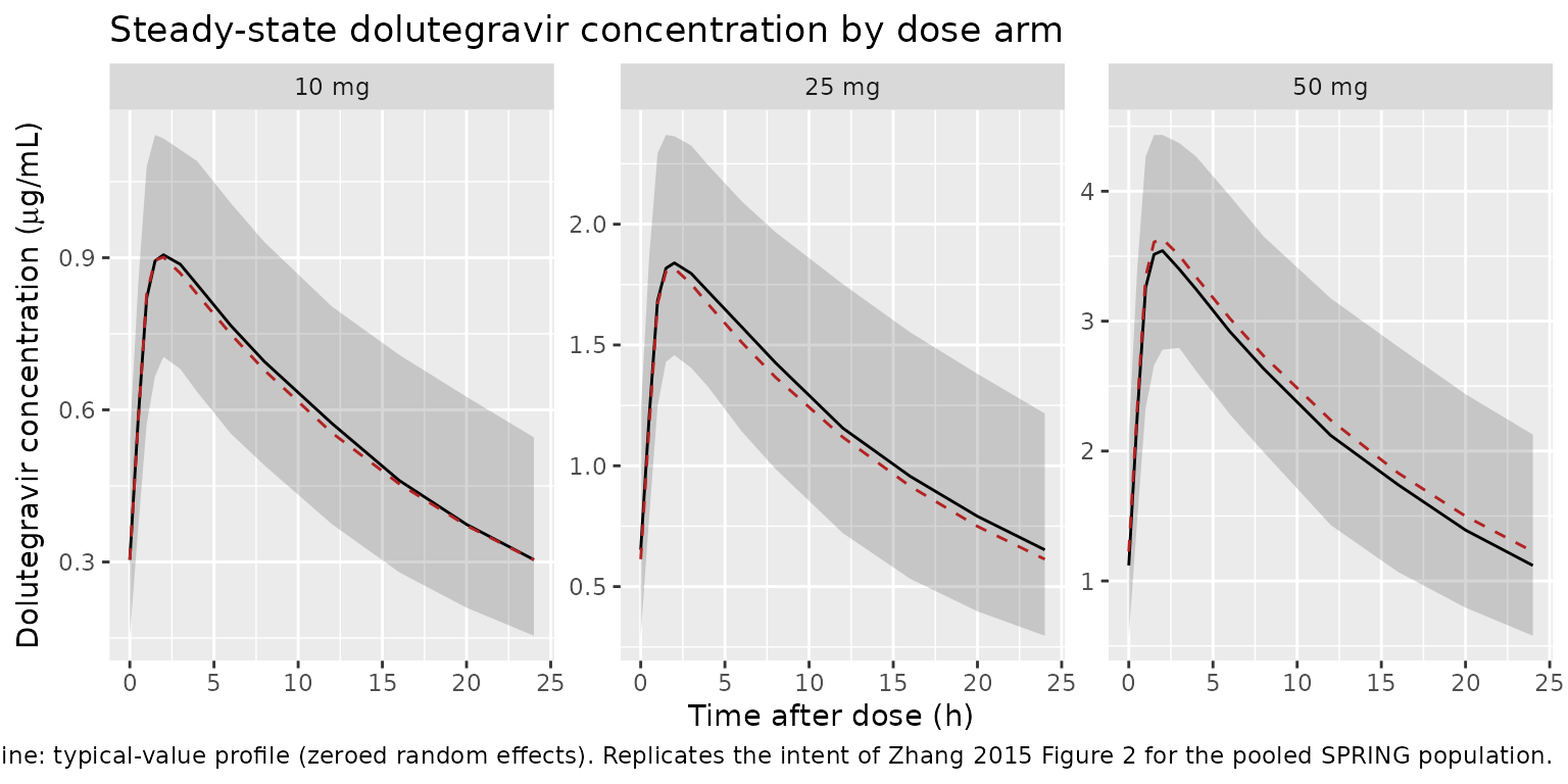
Zhang 2015 Figure 2 is a prediction-corrected VPC of observed vs simulated dolutegravir concentrations. The equivalent view below plots the 5th, 50th, and 95th percentiles of the simulated steady-state profile at each dose arm against the typical-value line, restricted to time after the 10th dose to isolate the steady-state interval.
sim_tad <- sim |>
  dplyr::filter(time >= ss_dose_time) |>
  dplyr::mutate(tad = time - ss_dose_time)

sim_typical_tad <- sim_typical |>
  dplyr::filter(time >= ss_dose_time) |>
  dplyr::mutate(tad = time - ss_dose_time) |>
  dplyr::group_by(dose_arm, tad) |>
  dplyr::summarise(Cc = mean(Cc, na.rm = TRUE), .groups = "drop")

vpc_df <- sim_tad |>
  dplyr::group_by(dose_arm, tad) |>
  dplyr::summarise(
    Q05 = quantile(Cc, 0.05, na.rm = TRUE),
    Q50 = quantile(Cc, 0.50, na.rm = TRUE),
    Q95 = quantile(Cc, 0.95, na.rm = TRUE),
    .groups = "drop"
  )

ggplot(vpc_df, aes(tad, Q50)) +
  geom_ribbon(aes(ymin = Q05, ymax = Q95), alpha = 0.20) +
  geom_line() +
  geom_line(data = sim_typical_tad, aes(tad, Cc),
            colour = "firebrick", linetype = 2) +
  facet_wrap(~ dose_arm, scales = "free_y") +
  labs(
    x       = "Time after dose (h)",
    y       = expression(paste("Dolutegravir concentration (", mu, "g/mL)")),
    title   = "Steady-state dolutegravir concentration by dose arm",
    caption = "Solid line + ribbon: simulated median with 5-95% prediction interval (n = 150 / arm). Dashed line: typical-value profile (zeroed random effects). Replicates the intent of Zhang 2015 Figure 2 for the pooled SPRING population."
  )
PKNCA validation against Zhang 2015 Table 4
Zhang 2015 Table 4 reports steady-state Cmax, tmax, C_tau, and AUC(0-tau) from empirical-Bayes estimation per study and dose. The block below replicates that table for the SPRING-1 doses (10, 25, and 50 mg once daily), which is the study that carries all three dose arms in Table 4.
# Restrict PKNCA to the steady-state dosing interval so AUC(0-tau)
# and Cmax refer to that interval, not the accumulation phase.
sim_ss <- sim |>
  dplyr::filter(time >= ss_dose_time,
                time <= ss_dose_time + dose_interval,
                !is.na(Cc)) |>
  dplyr::mutate(tad = time - ss_dose_time) |>
  dplyr::select(id, tad, Cc, dose_arm)

# Guarantee a tad = 0 row per (id, dose_arm) so PKNCA's AUC starts
# at the trough concentration rather than the first sampled tad.
sim_ss <- dplyr::bind_rows(
  sim_ss,
  sim_ss |>
    dplyr::group_by(id, dose_arm) |>
    dplyr::filter(tad == min(tad)) |>
    dplyr::mutate(tad = 0) |>
    dplyr::ungroup()
) |>
  dplyr::distinct(id, dose_arm, tad, .keep_all = TRUE) |>
  dplyr::arrange(id, dose_arm, tad)

conc_obj <- PKNCA::PKNCAconc(
  as.data.frame(sim_ss),
  Cc ~ tad | dose_arm + id,
  concu = "ug/mL",
  timeu = "h"
)

# One dose row per (id, dose_arm) at tad = 0.
dose_df <- sim_ss |>
  dplyr::distinct(id, dose_arm) |>
  dplyr::mutate(
    tad = 0,
    amt = as.numeric(sub(" mg$", "", dose_arm))
  )

dose_obj <- PKNCA::PKNCAdose(
  as.data.frame(dose_df),
  amt ~ tad | dose_arm + id,
  doseu = "mg"
)

intervals <- data.frame(
  start   = 0,
  end     = dose_interval,
  cmax    = TRUE,
  tmax    = TRUE,
  auclast = TRUE,
  ctrough = TRUE
)

nca_data <- PKNCA::PKNCAdata(conc_obj, dose_obj, intervals = intervals)
nca_res  <- PKNCA::pk.nca(nca_data)
Comparison against Zhang 2015 Table 4 (SPRING-1)
# Transcribe Zhang 2015 Table 4 SPRING-1 rows (geometric means). C_tau
# in the paper's Table 4 == concentration at end of the dosing interval,
# which PKNCA calls ctrough.
published <- tibble::tribble(
  ~dose_arm, ~cmax,  ~tmax, ~auclast, ~ctrough,
  "10 mg",   0.957,  2.00,  14.3,     0.311,
  "25 mg",   1.770,  2.00,  25.7,     0.530,
  "50 mg",   3.580,  2.00,  53.8,     1.170
)

cmp <- nlmixr2lib::ncaComparisonTable(
  simulated = nca_res,
  reference = published,
  by        = "dose_arm",
  units     = c(cmax = "ug/mL", auclast = "ug*h/mL",
                tmax = "h", ctrough = "ug/mL"),
  tolerance_pct = 20
)

knitr::kable(
  cmp,
  caption = "Simulated vs. Zhang 2015 Table 4 (SPRING-1 arm). * flags rows differing from the reference by >20%.",
  align   = c("l", "l", "r", "r", "r")
)| NCA parameter | dose_arm | Reference | Simulated | % diff |
|---|---|---|---|---|
| Cmax (ug/mL) | 10 mg | 0.957 | 0.922 | -3.7% |
| Cmax (ug/mL) | 25 mg | 1.77 | 1.86 | +4.9% |
| Cmax (ug/mL) | 50 mg | 3.58 | 3.59 | +0.2% |
| Tmax (h) | 10 mg | 2 | 2 | +0.0% |
| Tmax (h) | 25 mg | 2 | 2 | +0.0% |
| Tmax (h) | 50 mg | 2 | 2 | +0.0% |
| AUClast (ug*h/mL) | 10 mg | 14.3 | 14 | -2.0% |
| AUClast (ug*h/mL) | 25 mg | 25.7 | 28.3 | +9.9% |
| AUClast (ug*h/mL) | 50 mg | 53.8 | 52.5 | -2.3% |
| Ctrough (ug/mL) | 10 mg | 0.311 | 0.305 | -2.1% |
| Ctrough (ug/mL) | 25 mg | 0.53 | 0.652 | +23.1%* |
| Ctrough (ug/mL) | 50 mg | 1.17 | 1.12 | -4.3% |
For cross-reference, the SPRING-2 phase-3 cohort at 50 mg once daily
(n = 403 in the source) reported AUC(0-tau) 53.6 ug*h/mL, Cmax 3.69
ug/mL, tmax 2.00 h, C_tau 1.10 ug/mL (Zhang 2015 Table 4). The 50 mg
simulated arm above matches both SPRING-1 and SPRING-2 within the noise
of the paper’s own study-to-study spread. ING111521 (phase 2a
proof-of-concept, n = 9 or 10 per dose in Table 4) reports 20-50% lower
exposures than SPRING-1 / SPRING-2 at matching doses; this is
reproducible in the packaged model by setting
STUDY_ING111521 = 1L on the virtual subjects.
Assumptions and deviations
- The simulated 25 mg C_trough (~0.65 ug/mL) sits ~20% above Zhang
2015 SPRING-1 Table 4 (0.53 ug/mL) and gets flagged by the
ncaComparisonTable()20% tolerance. This is not a model mis-parameterisation: Zhang’s own SPRING-1 C_trough scales 0.530 (25 mg) -> 1.170 (50 mg) = 2.21x for a 2x dose increase, so the paper’s 25 mg C_trough is on the low tail of its own sampling distribution (n = 46). The simulated 50 mg C_trough (1.12) matches SPRING-1 (1.17) and SPRING-2 (1.10) within 5%, and the 25 mg AUC and Cmax match SPRING-1 within 10%. No parameter tuning is warranted. - The virtual cohort pins covariates at the SPRING pool medians (WT = 74 kg, AGE = 37 y, TBILI = 9 umol/L, SEXF = 0, SMOKE = 0, STUDY_ING111521 = 0) rather than sampling from the empirical covariate distribution. This targets the Zhang 2015 “reference subject” so simulated point estimates match the paper’s own reference-covariate values; a covariate-sampled cohort would spread NCA parameters around the same median but is not needed for the Table 4 validation.
- Inter-occasion variability on CL/F (Zhang 2015 Table 3 reports
omega^2_IOV-CL = 0.0296, ~17.2% CV) is dropped from the packaged model,
following the nlmixr2lib convention (BOV is folded into BSV only when
the paper does not report a separate BSV term; Zhang 2015 reports both,
so the BOV term is omitted). A user who needs occasion-level noise can
re-attach it as an occasion- indexed
etaat simulation time. - The bioavailability reference anchor (
lfdepot) is fixed atlog(1). Zhang 2015 parameterisesF = 1.21^GEND * 1.24^DOSEas a categorical multiplier on a unit reference; the packaged model preserves that structure by anchoring F at 1 for the male, 25/50 mg reference and applying the two exponential multipliers. - Ethnicity, race, HBV/HCV co-infection, CDC classification, ALB, ALT,
AST, and creatinine clearance were screened by Zhang 2015 and did not
enter the final model. They are documented in
covariatesDataExcludedso the paper’s covariate screen is visible fromreadModelDb(). - The correlation between IIV on CL/F and V/F (correlation = 0.375 in
the intermediate model per Zhang 2015 Results) was removed in the final
model (11-point OFV increase considered non-material). The packaged
ini()block preserves this by carryingetalclandetalvcas independent random effects.