Furosemide (Hornik 2025) • nlmixr2lib

Model and source

#> ℹ parameter labels from comments will be replaced by 'label()'

Citation: Hornik CP, Foote HP, Kendig E, Mohr J. An Adult Population Pharmacokinetic Model to Simulate Subcutaneous Administration of a Fixed Dose of Furosemide in Adolescents with Heart Failure and Volume Overload. Clin Pharmacokinet. 2025;64:899-908. doi:10.1007/s40262-025-01515-2
Description: Two-compartment population PK model with first-order subcutaneous absorption for furosemide in adults with chronic heart failure and volume overload, allometrically scaled to adolescents (Hornik 2025)
Article: https://doi.org/10.1007/s40262-025-01515-2
Supplement (Table S1, Figures S1-S8): https://doi.org/10.1007/s40262-025-01515-2 (electronic supplementary material)

Hornik and colleagues developed an adult population PK model for furosemide from a randomized crossover study comparing a buffered subcutaneous formulation (Furoscix, delivered by a wearable On-Body Infusor) against intravenous furosemide, then scaled that model allometrically to predict exposure in adolescents receiving the fixed 80 mg subcutaneous regimen.

Population

The adult model was built on 15 adults with chronic heart failure (NYHA class II/III) and chronic volume overload enrolled in NCT02329834 (Sect. 2.1, Sect. 3.1). Sixteen adults received furosemide; one was excluded for high pre-dose furosemide concentrations. Median age was 69 years (range 52-83) and 14 of 15 (93.3%) were men. Each patient received both treatments in a crossover with a 7-day washout: 80 mg subcutaneously (30 mg over the first 60 min, then 12.5 mg/h for 4 h) and 80 mg intravenously (40 mg over 2 min, repeated 2 h later). Median sampling was 21 samples per patient on the intravenous occasion and 18 on the subcutaneous occasion.

The paper reports no baseline demographics table, so weight, body mass index and renal function are available only from the axes of the ETA-versus-covariate panels in the supplement (Figures S1-S5): weight roughly 60-120 kg, creatinine clearance roughly 60-140 mL/min/1.73 m^2, body mass index roughly 25-35 kg/m^2 and serum creatinine roughly 1.0-1.8 mg/dL. The median renal function used as the covariate reference is 86 (Sect. 2.6).

str(readModelDb("Hornik_2025_furosemide")()$population)
#> List of 14
#>  $ species       : chr "human"
#>  $ n_subjects    : num 15
#>  $ n_studies     : num 1
#>  $ age_range     : chr "52-83 years"
#>  $ age_median    : chr "69 years"
#>  $ weight_range  : chr "approximately 60-120 kg (not tabulated in the paper; read from the weight axis of ETA-versus-covariate Figures S1-S5)"
#>  $ weight_median : chr "not reported"
#>  $ sex_female_pct: num 6.7
#>  $ race_ethnicity: chr "not reported"
#>  $ disease_state : chr "chronic heart failure, NYHA class II/III, with chronic volume overload requiring oral furosemide >= 40 mg/day f"| __truncated__
#>  $ renal_function: chr "median eGFR 86 mL/min (Cockcroft-Gault); observed range approximately 60-140 mL/min/1.73 m^2 from Figures S1-S5"
#>  $ dose_range    : chr "80 mg subcutaneous (30 mg over the first 60 min then 12.5 mg/h for 4 h) and 80 mg intravenous (40 mg over 2 min"| __truncated__
#>  $ regions       : chr "USA (single site)"
#>  $ notes         : chr "Adult analysis population of NCT02329834 (Sect. 2.1, Sect. 3.1). Sixteen adults received furosemide; one was ex"| __truncated__

Source trace

Every ini() entry in inst/modeldb/specificDrugs/Hornik_2025_furosemide.R carries an in-file comment naming its origin. They are collected here for review. Equation numbers are those of the published article.

Equation / parameter	Value	Source location
`lka` (Ka)	1.30 1/h	Table 1, “K a , h-1”; structure Eq. 14
`lcl` (CL)	6.51 L/h	Table 1, “CL, L/h”; structure Eq. 15
`lvc` (Vc)	5.37 L	Table 1, “V c , L”; structure Eq. 16
`lq` (Q)	3.74 L/h	Table 1, “Q , L/h”; structure Eq. 17
`lvp` (Vp)	5.95 L	Table 1, “V p , L”; structure Eq. 18
`lfdepot` (F, subcutaneous)	0.96	Sect. 3.2 text; logit form Eq. 19. Not in Table 1 – see “Reconciling the reported bioavailability” below
`e_crcl_cl`	0.74	Table 1, “eGFR on CL”; power form Eq. 15, reference 86
`e_wt_cl_q`	0.75 (fixed)	Eqs. 10 and 12; held at the conventional value per Sect. 2.6 and Sect. 4
`e_wt_vc_vp`	1 (fixed)	Eqs. 11 and 13
`etalka`	21.7% CV	Table 1, IIV block (shrinkage 10%)
`etalcl`	18.5% CV	Table 1, IIV block (shrinkage 0%)
`etalvc`	31.7% CV	Table 1, IIV block (shrinkage 0%)
`etalq`	33.1% CV	Table 1, IIV block (shrinkage 6%)
`etalvp`	18.9% CV	Table 1, IIV block (shrinkage 3%)
`propSd`	0.126	Table 1, “Proportional error, %” = 12.6%; combined form Eq. 5
`addSd`	0.100 ug/mL	Table 1, “Additive error, ng/mL” = 100 ng/mL
Exponential IIV, `exp(eta)`	n/a	Eq. 1
Combined residual error	n/a	Eq. 5
Two-compartment ODEs with first-order subcutaneous absorption	n/a	Sect. 3.2 (“two-compartment model with linear kinetics and a first-order absorption rate constant”)
Allometric scaling to 70 kg	n/a	Eqs. 9-13

Covariate effects that were screened but not retained (age on Vp, serum creatinine, body mass index, sex, NYHA class) are recorded in the model file’s covariatesDataExcluded metadata rather than implemented; the covariate search is Table S1 and Figures S1-S5 of the supplement.

The IIV variances are stored on the variance scale as omega^2 = log(CV^2 + 1):

tibble::tibble(
  parameter = c("etalka", "etalcl", "etalvc", "etalq", "etalvp"),
  cv_pct    = c(21.7, 18.5, 31.7, 33.1, 18.9)
) |>
  dplyr::mutate(omega_sq = round(log((cv_pct / 100)^2 + 1), 6)) |>
  dplyr::rename("Parameter" = parameter, "Table 1 CV%" = cv_pct,
                "omega^2 in ini()" = omega_sq) |>
  knitr::kable(caption = "Table 1 CV% converted to the variance scale.")

Table 1 CV% converted to the variance scale.
Parameter	Table 1 CV%	omega^2 in ini()
etalka	21.7	0.046014
etalcl	18.5	0.033652
etalvc	31.7	0.095755
etalq	33.1	0.103964
etalvp	18.9	0.035098

Virtual cohort

The original observed concentrations are not public. The simulations below rebuild the paper’s virtual adolescent population (Sect. 2.7): three weight bands (42.5-50.0, >50-60 and >60-70 kg) with weight distributed uniformly within each band, plus a typical 70 kg adult reference. Renal function is fixed at the adult population median of 86 for every virtual subject, which is what the authors did – Sect. 4 states the pediatric parameters were fixed at “the population parameter estimate of a 70-kg adult with an eGFR of 86 mL/min”. Between-subject variability is switched off, again matching Sect. 2.7 (“To represent the anticipated exposures in typical adolescents within a given weight group, IIV was not included in the simulations”), so the only source of spread within a band is body weight.

The paper simulated 1000 virtual adolescents per band; 200 per arm is used here (the library cap), which is more than sufficient because the weight grid is deterministic.

set.seed(20250513)

n_per_band <- 200L

bands <- tibble::tribble(
  ~grp,             ~wt_lo, ~wt_hi,
  "42.5-50.0 kg",    42.5,   50.0,
  ">50-60 kg",       50.0,   60.0,
  ">60-70 kg",       60.0,   70.0,
  "Adult (70 kg)",   70.0,   70.0
)

# Observations every 0.1 h to 24 h (the paper's grid, Sect. 2.7). The grid is
# extended to 72 h at a coarser spacing so the AUC mass-balance identity below
# can be checked over a practically infinite window; the 0-24 h interval used
# for the comparison against Table 2 is unaffected.
obs_times <- c(seq(0, 24, by = 0.1), seq(24.5, 72, by = 0.5))

make_band <- function(grp, wt_lo, wt_hi, id_offset) {
  wt <- if (isTRUE(all.equal(wt_lo, wt_hi))) {
    rep(wt_lo, n_per_band)
  } else {
    seq(wt_lo, wt_hi, length.out = n_per_band)
  }
  subj <- tibble::tibble(
    id   = id_offset + seq_len(n_per_band),
    WT   = wt,
    CRCL = 86,
    grp  = grp
  )
  # 80 mg subcutaneously: 30 mg over the first hour, then 12.5 mg/h for 4 h.
  # `dur` (not `rate`) is used so bioavailability scales the delivered rate
  # while the pump's programmed duration stays fixed.
  doses <- dplyr::bind_rows(
    dplyr::mutate(subj, time = 0, amt = 30, evid = 1L, dur = 1, cmt = "depot"),
    dplyr::mutate(subj, time = 1, amt = 50, evid = 1L, dur = 4, cmt = "depot")
  )
  obs <- tidyr::crossing(subj, time = obs_times) |>
    dplyr::mutate(amt = NA_real_, evid = 0L, dur = NA_real_, cmt = "central")
  dplyr::bind_rows(doses, obs) |>
    dplyr::arrange(id, time, dplyr::desc(evid))
}

events <- dplyr::bind_rows(
  lapply(seq_len(nrow(bands)), function(i) {
    make_band(bands$grp[i], bands$wt_lo[i], bands$wt_hi[i],
              id_offset = (i - 1L) * 1000L)
  })
)

stopifnot(!anyDuplicated(unique(events[, c("id", "time", "evid")])))
stopifnot(nrow(dplyr::distinct(events, id)) == 4L * n_per_band)

Each band’s dosing totals the fixed 80 mg regimen:

events |>
  dplyr::filter(evid == 1) |>
  dplyr::group_by(grp, id) |>
  dplyr::summarise(total_dose_mg = sum(amt), .groups = "drop") |>
  dplyr::group_by(grp) |>
  dplyr::summarise(total_dose_mg = mean(total_dose_mg), .groups = "drop") |>
  dplyr::rename("Weight band" = grp, "Total dose (mg)" = total_dose_mg) |>
  knitr::kable(caption = "Fixed 80 mg subcutaneous dose in every band.")

Fixed 80 mg subcutaneous dose in every band.
Weight band	Total dose (mg)
42.5-50.0 kg	80
>50-60 kg	80
>60-70 kg	80
Adult (70 kg)	80

Simulation

mod <- readModelDb("Hornik_2025_furosemide")

# Sect. 2.7: IIV was excluded from the dosing simulations.
mod_typical <- rxode2::zeroRe(mod)
#> ℹ parameter labels from comments will be replaced by 'label()'

sim <- rxode2::rxSolve(
  mod_typical, events = events,
  keep = c("WT", "grp"),
  returnType = "data.frame"
) |>
  as.data.frame()
#> ℹ omega/sigma items treated as zero: 'etalka', 'etalcl', 'etalvc', 'etalq', 'etalvp'
#> Warning: multi-subject simulation without without 'omega'

stopifnot(dplyr::n_distinct(sim$id) == 4L * n_per_band)

With the random effects zeroed, two subjects at the same weight must give identical predictions – the adult band is 200 copies of a 70 kg subject, so its spread must be exactly zero:

adult_cmax <- sim |>
  dplyr::filter(grp == "Adult (70 kg)", !is.na(Cc)) |>
  dplyr::group_by(id) |>
  dplyr::summarise(cmax = max(Cc), .groups = "drop")

stopifnot(nrow(adult_cmax) == n_per_band)
stopifnot(diff(range(adult_cmax$cmax)) == 0)
cat("Adult band spread in Cmax:", diff(range(adult_cmax$cmax)), "ug/mL\n")
#> Adult band spread in Cmax: 0 ug/mL

Replicate published figures

sim |>
  dplyr::filter(!is.na(Cc), time <= 24) |>
  dplyr::group_by(grp, time) |>
  dplyr::summarise(
    Q05 = quantile(Cc, 0.05),
    Q50 = quantile(Cc, 0.50),
    Q95 = quantile(Cc, 0.95),
    .groups = "drop"
  ) |>
  ggplot(aes(time, Q50 * 1000, colour = grp, fill = grp)) +
  geom_ribbon(aes(ymin = Q05 * 1000, ymax = Q95 * 1000), alpha = 0.2,
              colour = NA) +
  geom_line(linewidth = 0.7) +
  labs(
    x = "Time since start of subcutaneous administration (h)",
    y = "Furosemide plasma concentration (ug/L)",
    colour = NULL, fill = NULL,
    title = "Figure 2 - simulated adolescent profiles versus a typical 70 kg adult",
    caption = "Replicates Figure 2 of Hornik 2025. Lines are medians; bands are the 5th-95th percentiles across body weight."
  ) +
  theme_bw() +
  theme(legend.position = "bottom")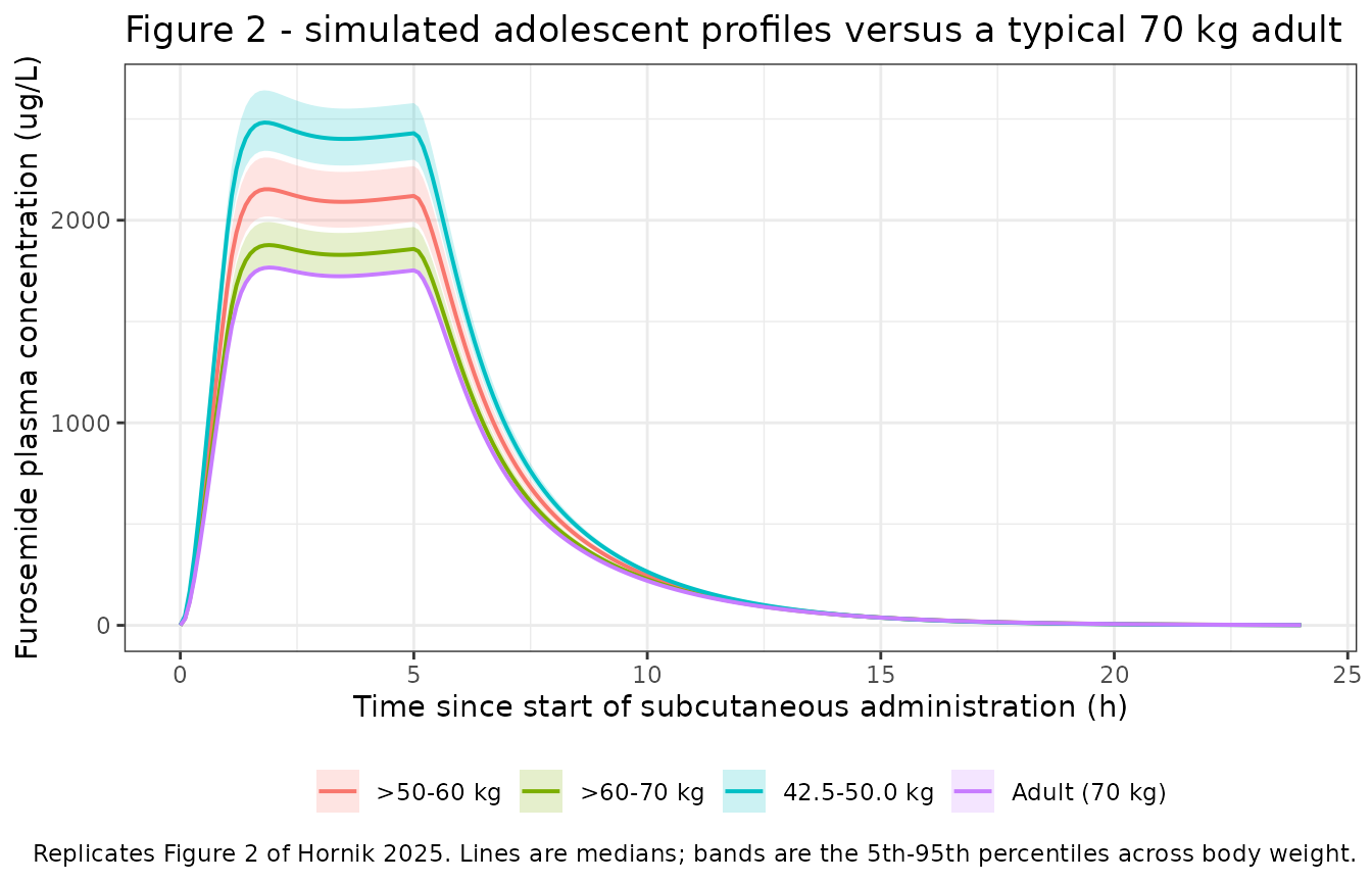

Replicates Figure 2 of Hornik 2025.

The shape matches the published figure: concentrations rise steeply during the 30 mg loading hour, peak shortly after the infusion steps down to 12.5 mg/h at 1 h, decline slowly through the remainder of the 5 h infusion, and then fall away once administration stops. Exposure increases as body weight decreases, because the dose is fixed while clearance scales with weight.

Structural identity check

Because clearance is linear and the dose is a finite infusion, total exposure must satisfy AUC(0-inf) = F * Dose / CL exactly for every subject. Checking this per subject, rather than comparing group medians, is a much stricter test: it exercises the allometric scaling, the bioavailability term and the two- compartment disposition together.

per_subject <- sim |>
  dplyr::filter(!is.na(Cc)) |>
  dplyr::group_by(id, grp, WT, cl) |>
  dplyr::summarise(
    auc_0_72 = sum(diff(time) * (head(Cc, -1) + tail(Cc, -1)) / 2),
    .groups  = "drop"
  ) |>
  dplyr::mutate(
    fdepot   = 0.96,
    expected = fdepot * 80 / cl,
    ratio    = auc_0_72 / expected
  )

summary(per_subject$ratio)
#>    Min. 1st Qu.  Median    Mean 3rd Qu.    Max. 
#>       1       1       1       1       1       1

# AUC(0-72 h) is a >30 half-life window, so the truncation loss is negligible.
stopifnot(all(abs(per_subject$ratio - 1) < 0.001))

Clearance itself must follow Eq. 10 exactly, CL = 6.51 * (WT/70)^0.75, since renal function is held at the reference value:

stopifnot(all(abs(per_subject$cl / (6.51 * (per_subject$WT / 70)^0.75) - 1) < 1e-8))

# Sect. 3.3 reports weight-normalized clearance of 1.55 mL/min/kg.
cl_norm_adult <- with(
  dplyr::filter(per_subject, grp == "Adult (70 kg)")[1, ],
  cl * 1000 / 60 / WT
)
cat(sprintf("Weight-normalized CL at 70 kg: %.3f mL/min/kg (paper: 1.55)\n",
            cl_norm_adult))
#> Weight-normalized CL at 70 kg: 1.550 mL/min/kg (paper: 1.55)
stopifnot(abs(cl_norm_adult - 1.55) < 0.005)

PKNCA validation

sim_nca <- sim |>
  dplyr::filter(!is.na(Cc)) |>
  dplyr::select(id, time, Cc, grp)

# Guarantee a time = 0 record per subject; pre-dose concentration is zero for
# this extravascular regimen.
sim_nca <- dplyr::bind_rows(
  sim_nca,
  sim_nca |> dplyr::distinct(id, grp) |> dplyr::mutate(time = 0, Cc = 0)
) |>
  dplyr::distinct(id, grp, time, .keep_all = TRUE) |>
  dplyr::arrange(id, grp, time)

conc_obj <- PKNCA::PKNCAconc(
  sim_nca, Cc ~ time | grp + id,
  concu = "ug/mL", timeu = "h"
)

dose_df <- events |>
  dplyr::filter(evid == 1) |>
  dplyr::select(id, time, amt, grp)

dose_obj <- PKNCA::PKNCAdose(dose_df, amt ~ time | grp + id, doseu = "mg")

# Sect. 2.7 / Table 2 report AUC(0-24) and Cmax over the 24 h window.
intervals <- data.frame(
  start     = 0,
  end       = 24,
  cmax      = TRUE,
  tmax      = TRUE,
  auclast   = TRUE,
  half.life = TRUE
)

nca_res <- PKNCA::pk.nca(
  PKNCA::PKNCAdata(conc_obj, dose_obj, intervals = intervals)
)

nca_res$result |>
  dplyr::filter(PPTESTCD %in% c("cmax", "tmax", "auclast", "half.life")) |>
  dplyr::group_by(grp, PPTESTCD) |>
  dplyr::summarise(
    geomean = exp(mean(log(PPORRES))),
    cv_pct  = sqrt(exp(stats::var(log(PPORRES))) - 1) * 100,
    .groups = "drop"
  ) |>
  dplyr::mutate(
    PPTESTCD = nlmixr2lib::ncaParamLabel(PPTESTCD),
    geomean  = signif(geomean, 4),
    cv_pct   = round(cv_pct, 2)
  ) |>
  dplyr::rename("Weight band" = grp, "NCA parameter" = PPTESTCD,
                "Geometric mean" = geomean, "CV%" = cv_pct) |>
  knitr::kable(caption = "Simulated NCA over 0-24 h (Cc in ug/mL, time in h).")

Simulated NCA over 0-24 h (Cc in ug/mL, time in h).
Weight band	NCA parameter	Geometric mean	CV%
42.5-50.0 kg	AUClast	16.110	3.55
42.5-50.0 kg	Cmax	2.485	3.88
42.5-50.0 kg	t½	1.782	1.19
42.5-50.0 kg	Tmax	1.800	0.00
>50-60 kg	AUClast	14.150	3.98
>50-60 kg	Cmax	2.156	4.35
>50-60 kg	t½	1.861	1.32
>50-60 kg	Tmax	1.867	2.54
>60-70 kg	AUClast	12.480	3.36
>60-70 kg	Cmax	1.879	3.68
>60-70 kg	t½	1.941	1.11
>60-70 kg	Tmax	1.900	0.00
Adult (70 kg)	AUClast	11.790	0.00
Adult (70 kg)	Cmax	1.767	0.00
Adult (70 kg)	t½	1.978	0.00
Adult (70 kg)	Tmax	1.900	0.00

Comparison against published NCA

Table 2 of Hornik 2025 reports AUC(0-24) in ugh/L and Cmax in ug/L. The model works in ug/mL (dose in mg, volumes in L), so the published values are divided by 1000 below: 16,800 ugh/L is 16.8 ug*h/mL, 2590 ug/L is 2.59 ug/mL, and so on.

published <- tibble::tribble(
  ~grp,             ~auclast, ~cmax,
  "42.5-50.0 kg",   16.8,     2.590,
  ">50-60 kg",      14.7,     2.240,
  ">60-70 kg",      13.0,     1.960,
  "Adult (70 kg)",  12.4,     1.900
)

cmp <- nlmixr2lib::ncaComparisonTable(
  simulated     = nca_res,
  reference     = published,
  by            = "grp",
  units         = c(cmax = "ug/mL", auclast = "ug*h/mL"),
  tolerance_pct = 20
)

knitr::kable(
  cmp,
  caption = "Simulated versus Table 2 of Hornik 2025. * differs from reference by >20%.",
  align   = c("l", "l", "r", "r", "r")
)

Simulated versus Table 2 of Hornik 2025. * differs from reference by >20%.
NCA parameter	grp	Reference	Simulated	% diff
Cmax (ug/mL)	42.5-50.0 kg	2.59	2.48	-4.2%
Cmax (ug/mL)	>50-60 kg	2.24	2.15	-3.9%
Cmax (ug/mL)	>60-70 kg	1.96	1.88	-4.2%
Cmax (ug/mL)	Adult (70 kg)	1.9	1.77	-7.0%
AUClast (ug*h/mL)	42.5-50.0 kg	16.8	16.1	-4.2%
AUClast (ug*h/mL)	>50-60 kg	14.7	14.1	-3.9%
AUClast (ug*h/mL)	>60-70 kg	13	12.5	-4.1%
AUClast (ug*h/mL)	Adult (70 kg)	12.4	11.8	-4.9%

No row exceeds the 20% tolerance. Every simulated value nonetheless sits below the published one, and across the three adolescent bands the shortfall is close to 4% and near-identical for AUC and for Cmax – the signature of a single multiplicative factor rather than a structural disagreement. That factor is bioavailability, as the next section shows. The adult row is the exception (about 5% low on AUC but 7% low on Cmax); it is a different kind of target, for the reason given at the end of that section.

Reconciling the reported bioavailability

Section 3.2 states that “bioavailability following subcutaneous furosemide administration was estimated at 0.96”, and that is the value packaged in the model. Table 1 does not list the corresponding theta(6), so 0.96 is the only published number for this parameter.

The paper’s own simulations, however, are only reproducible with F = 1. Two independent internal checks establish this.

First, clearance is pinned by Sect. 3.3: the reported weight-normalized clearance of 1.55 mL/min/kg is exactly 6.51 L/h / 70 kg, confirming that the simulations used the Table 1 estimate of 6.51 L/h and the 70 kg reference.

Second, with clearance fixed, AUC(0-24) ~ F * Dose / CL back-solves bioavailability directly from each published exposure. Since the truncation loss over 24 h is negligible (below), the arithmetic is essentially exact:

band_gm_wt <- function(a, b) {
  if (isTRUE(all.equal(a, b))) return(a)
  exp((b * log(b) - b - a * log(a) + a) / (b - a))  # geometric mean of U(a, b)
}

backsolve_f <- bands |>
  dplyr::mutate(
    gm_wt     = mapply(band_gm_wt, wt_lo, wt_hi),
    cl        = 6.51 * (gm_wt / 70)^0.75,
    published = c(16.8, 14.7, 13.0, 12.4),          # ug*h/mL, Table 2
    f_implied = published * cl / 80
  )

backsolve_f |>
  dplyr::mutate(dplyr::across(c(gm_wt, cl, f_implied), \(x) round(x, 3))) |>
  dplyr::select(grp, gm_wt, cl, published, f_implied) |>
  dplyr::rename(
    "Weight band"                = grp,
    "Geometric mean weight (kg)" = gm_wt,
    "CL (L/h)"                   = cl,
    "Published AUC0-24 (ug*h/mL)" = published,
    "Implied F"                  = f_implied
  ) |>
  knitr::kable(caption = "Bioavailability back-solved from Table 2.")

Bioavailability back-solved from Table 2.
Weight band	Geometric mean weight (kg)	CL (L/h)	Published AUC0-24 (ug*h/mL)	Implied F
42.5-50.0 kg	46.199	4.767	16.8	1.001
>50-60 kg	54.924	5.427	14.7	0.997
>60-70 kg	64.936	6.153	13.0	1.000
Adult (70 kg)	70.000	6.510	12.4	1.009

The three adolescent bands – where Sect. 2.7 guarantees that weight is the only source of variation – all return F within a fraction of a percent of 1.00, not 0.96. Rescaling the simulated exposures by 1 / 0.96 therefore reproduces Table 2 almost exactly:

rescaled <- nca_res$result |>
  dplyr::filter(PPTESTCD %in% c("auclast", "cmax")) |>
  dplyr::group_by(grp, PPTESTCD) |>
  dplyr::summarise(
    geomean = exp(mean(log(PPORRES))),
    cv_pct  = sqrt(exp(stats::var(log(PPORRES))) - 1) * 100,
    .groups = "drop"
  ) |>
  dplyr::mutate(at_f1 = geomean / 0.96) |>
  dplyr::left_join(
    published |>
      tidyr::pivot_longer(c(auclast, cmax), names_to = "PPTESTCD",
                          values_to = "reference"),
    by = c("grp", "PPTESTCD")
  ) |>
  dplyr::mutate(
    pct_diff_at_f096 = 100 * (geomean / reference - 1),
    pct_diff_at_f1   = 100 * (at_f1 / reference - 1),
    PPTESTCD         = nlmixr2lib::ncaParamLabel(PPTESTCD)
  )

rescaled |>
  dplyr::mutate(dplyr::across(c(geomean, at_f1, reference), \(x) signif(x, 4)),
                dplyr::across(dplyr::starts_with("pct_diff"), \(x) round(x, 2)),
                cv_pct = round(cv_pct, 2)) |>
  dplyr::select(grp, PPTESTCD, reference, geomean, pct_diff_at_f096,
                at_f1, pct_diff_at_f1, cv_pct) |>
  dplyr::rename(
    "Weight band"        = grp,
    "NCA parameter"      = PPTESTCD,
    "Published"          = reference,
    "Simulated (F=0.96)" = geomean,
    "% diff (F=0.96)"    = pct_diff_at_f096,
    "Simulated (F=1.00)" = at_f1,
    "% diff (F=1.00)"    = pct_diff_at_f1,
    "Simulated CV%"      = cv_pct
  ) |>
  knitr::kable(caption = "Published Table 2 versus the packaged model at F = 0.96 and rescaled to F = 1.00.")

Published Table 2 versus the packaged model at F = 0.96 and rescaled to F = 1.00.
Weight band	NCA parameter	Published	Simulated (F=0.96)	% diff (F=0.96)	Simulated (F=1.00)	% diff (F=1.00)	Simulated CV%
42.5-50.0 kg	AUClast	16.80	16.110	-4.12	16.780	-0.13	3.55
42.5-50.0 kg	Cmax	2.59	2.485	-4.07	2.588	-0.07	3.88
>50-60 kg	AUClast	14.70	14.150	-3.77	14.740	0.24	3.98
>50-60 kg	Cmax	2.24	2.156	-3.77	2.245	0.24	4.35
>60-70 kg	AUClast	13.00	12.480	-4.03	13.000	-0.03	3.36
>60-70 kg	Cmax	1.96	1.879	-4.13	1.957	-0.14	3.68
Adult (70 kg)	AUClast	12.40	11.790	-4.90	12.280	-0.94	0.00
Adult (70 kg)	Cmax	1.90	1.767	-7.02	1.840	-3.15	0.00

# Every adolescent band agrees with Table 2 to better than 0.5% once F = 1,
# and is uniformly ~4% low at F = 0.96.
adolescent <- dplyr::filter(rescaled, grp != "Adult (70 kg)")
stopifnot(all(abs(adolescent$pct_diff_at_f1) < 0.5))
stopifnot(all(abs(adolescent$pct_diff_at_f096 + 4.17) < 0.6))

The published CV% values corroborate the reconstruction independently of the bioavailability question, because a scale factor cannot change a coefficient of variation. Table 2 reports AUC CV% of 3.51, 3.92 and 3.26 and Cmax CV% of 3.84, 4.28 and 3.58 for the three adolescent bands; the simulated CV% in the table above match those to within about 0.1 percentage point, which confirms the uniform-within-band weight distribution and the 0.75 allometric exponent. That agreement is asserted here rather than left as a prose claim:

published_cv <- tibble::tribble(
  ~grp,           ~PPTESTCD, ~reference_cv,   # Table 2, CV% in parentheses
  "42.5-50.0 kg", "AUClast", 3.51,
  ">50-60 kg",    "AUClast", 3.92,
  ">60-70 kg",    "AUClast", 3.26,
  "42.5-50.0 kg", "Cmax",    3.84,
  ">50-60 kg",    "Cmax",    4.28,
  ">60-70 kg",    "Cmax",    3.58
)

cv_check <- rescaled |>
  dplyr::inner_join(published_cv, by = c("grp", "PPTESTCD")) |>
  dplyr::mutate(cv_diff_pp = cv_pct - reference_cv)

# Guard against a silently empty join before testing the values themselves.
stopifnot(nrow(cv_check) == nrow(published_cv))
stopifnot(all(abs(cv_check$cv_diff_pp) < 0.12))

The adult row is the one group that does not tighten under F = 1 (about 1% low on AUC and 3% low on Cmax). That is expected: Table 2 reports CV% of 18.70 for adult AUC and 14.50 for adult Cmax, whereas a single typical 70 kg adult with the reference renal function has a CV of exactly zero (verified above). The adult column was therefore evidently simulated across the observed adult covariate distribution rather than at a single typical value, so it is not a like-for-like target for a typical-value replication.

Because the two candidate values cannot be separated from the paper alone – the printed 0.96 may be a typographical slip for 0.996 (the pivotal PK study cited in the Introduction reported 99.6% bioavailability for this formulation and regimen), or the simulation code may simply not have applied F – the model ships the value the paper actually prints for the parameter. Users who want to reproduce Table 2 exactly can override it:

mod_f1 <- readModelDb("Hornik_2025_furosemide") |>
  rxode2::ini(lfdepot = log(1))

Adult model with between-subject variability

The dosing simulations above exclude IIV by design. The final adult model does carry inter-individual variability on all five structural parameters, so the block below exercises that path and shows the two administration routes side by side, as in the stratification of Figure 1. This is a forward simulation from the model, not a replication of Figure 1 – the observed concentrations that figure plots are not public.

set.seed(4242)
n_adult <- 200L

adult_subj <- tibble::tibble(id = seq_len(n_adult), WT = 70, CRCL = 86)
adult_obs_times <- seq(0, 24, by = 0.25)

adult_sc <- dplyr::bind_rows(
  dplyr::mutate(adult_subj, time = 0, amt = 30, evid = 1L, dur = 1, cmt = "depot"),
  dplyr::mutate(adult_subj, time = 1, amt = 50, evid = 1L, dur = 4, cmt = "depot"),
  tidyr::crossing(adult_subj, time = adult_obs_times) |>
    dplyr::mutate(amt = NA_real_, evid = 0L, dur = NA_real_, cmt = "central")
) |>
  dplyr::mutate(route = "Subcutaneous 80 mg")

# Intravenous arm: 40 mg over 2 min, repeated 2 h later (Sect. 2.1).
adult_iv <- dplyr::bind_rows(
  dplyr::mutate(adult_subj, time = 0, amt = 40, evid = 1L, dur = 2 / 60, cmt = "central"),
  dplyr::mutate(adult_subj, time = 2, amt = 40, evid = 1L, dur = 2 / 60, cmt = "central"),
  tidyr::crossing(adult_subj, time = adult_obs_times) |>
    dplyr::mutate(amt = NA_real_, evid = 0L, dur = NA_real_, cmt = "central")
) |>
  dplyr::mutate(id = id + 1000L, route = "Intravenous 40 mg x 2")

adult_events <- dplyr::bind_rows(adult_sc, adult_iv) |>
  dplyr::arrange(id, time, dplyr::desc(evid))

stopifnot(!anyDuplicated(unique(adult_events[, c("id", "time", "evid")])))

adult_sim <- rxode2::rxSolve(
  mod, events = adult_events,
  keep = c("route"),
  returnType = "data.frame"
) |>
  as.data.frame()
#> ℹ parameter labels from comments will be replaced by 'label()'

stopifnot(dplyr::n_distinct(adult_sim$id) == 2L * n_adult)

adult_sim |>
  dplyr::filter(!is.na(Cc), time > 0) |>
  dplyr::group_by(route, time) |>
  dplyr::summarise(
    Q05 = quantile(Cc, 0.05),
    Q50 = quantile(Cc, 0.50),
    Q95 = quantile(Cc, 0.95),
    .groups = "drop"
  ) |>
  ggplot(aes(time, Q50 * 1000)) +
  geom_ribbon(aes(ymin = Q05 * 1000, ymax = Q95 * 1000), alpha = 0.25) +
  geom_line(linewidth = 0.7) +
  facet_wrap(~route) +
  scale_y_log10() +
  labs(
    x = "Time after first dose (h)",
    y = "Furosemide plasma concentration (ug/L)",
    title = "Adult model with between-subject variability, by route",
    caption = "Median and 5th-95th percentiles, 200 virtual adults at 70 kg and the reference renal function."
  ) +
  theme_bw()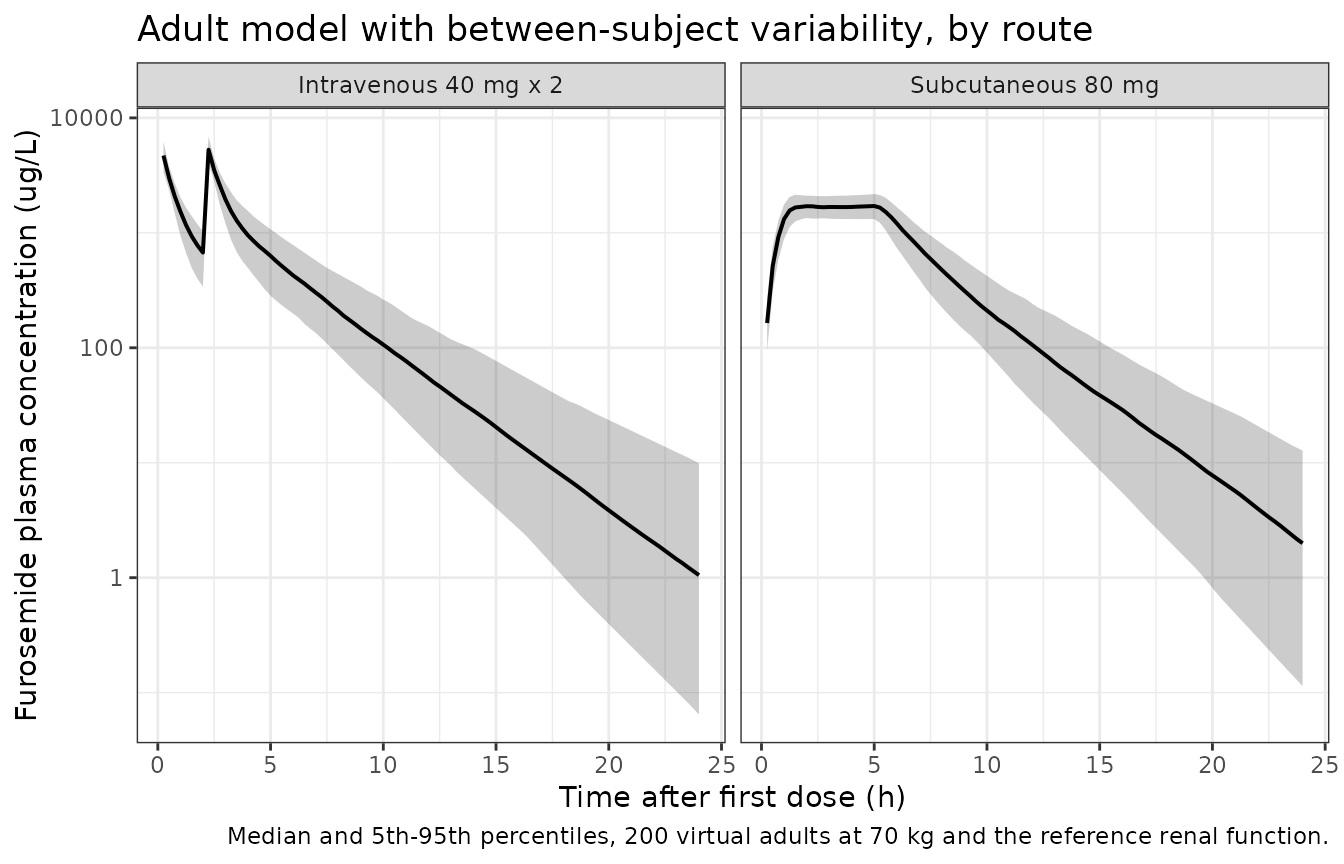

Simulated adult profiles by route, with between-subject variability (counterpart of the Figure 1 stratification).

The subcutaneous profile is flatter and more sustained than the intravenous profile, which is the pharmacokinetic rationale for the On-Body Infusor regimen described in Sect. 1.

Renal function is the model’s only retained covariate. Its effect on clearance follows Eq. 15 across the range observed in the adult study:

tibble::tibble(CRCL = seq(60, 140, by = 5)) |>
  dplyr::mutate(
    cl        = 6.51 * (CRCL / 86)^0.74,
    auc_ug_h_L = 0.96 * 80 / cl * 1000
  ) |>
  ggplot(aes(CRCL, cl)) +
  geom_line(linewidth = 0.7) +
  geom_vline(xintercept = 86, linetype = "dashed") +
  labs(
    x = "Creatinine clearance (mL/min/1.73 m^2)",
    y = "Clearance (L/h)",
    title = "Equation 15: renal function effect on clearance in a 70 kg adult",
    caption = "Dashed line marks the reference value of 86 used for normalization."
  ) +
  theme_bw()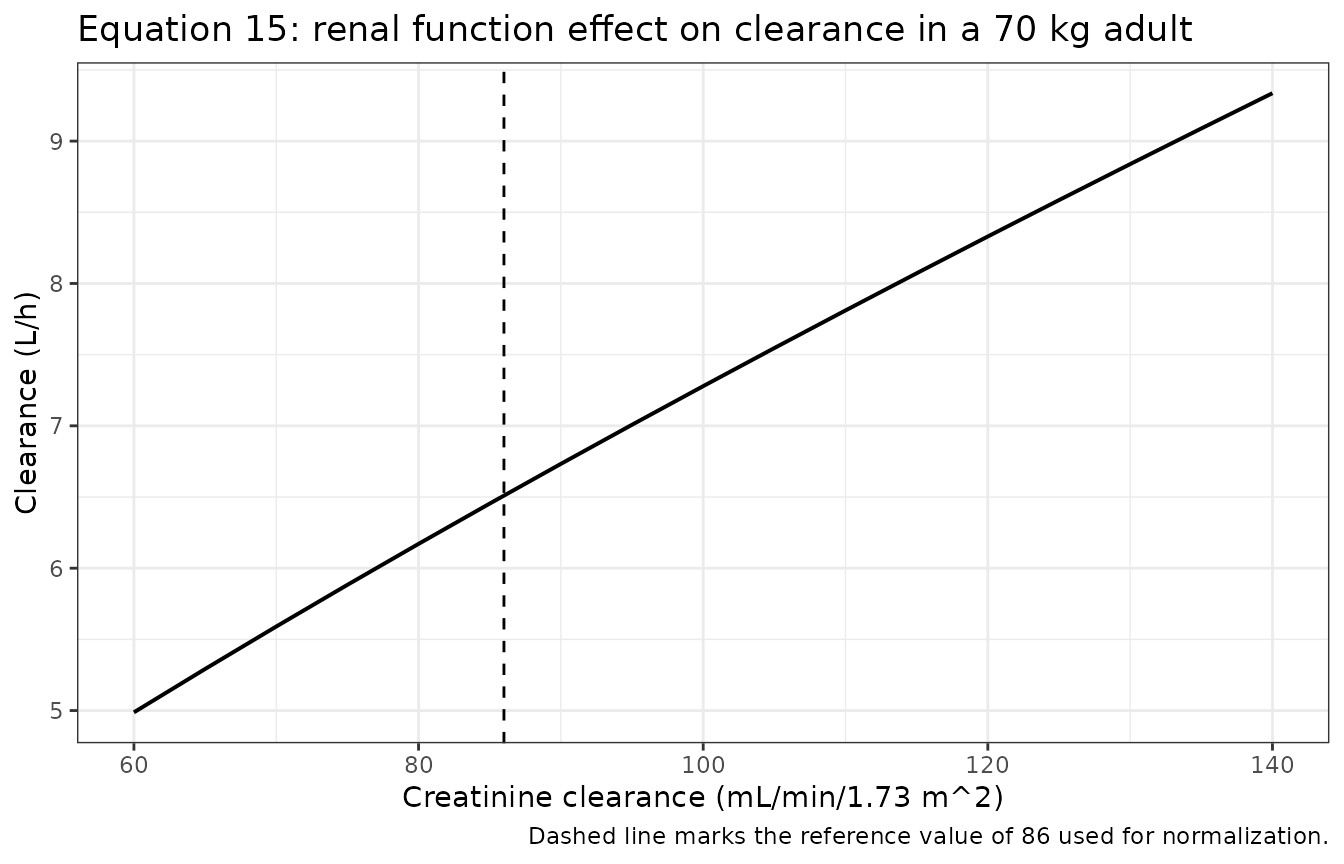

Assumptions and deviations

Bioavailability. The packaged lfdepot is the paper’s printed estimate of 0.96 (Sect. 3.2). The paper’s own Table 2 back-solves to F = 1.00, so every simulated exposure here is uniformly about 4% below the published value. The discrepancy is documented and quantified above rather than tuned away. Table 1 does not report theta(6), so 0.96 could not be cross-checked against the logit-scale estimate of Eq. 19.
Bioavailability parameterization. The paper estimates F on the logit scale (Eq. 19). The model file uses the library’s canonical lfdepot (log scale) at the same point estimate; the two parameterizations differ only in the estimation transform, not in the predicted value.
Weight in the adult model. Weight was screened but not retained as a covariate in the adult fit (Sect. 3.2, Table S1). The allometric terms in the model file are the authors’ Eqs. 9-13, which they applied post hoc to extrapolate the adult model to adolescents. Both size terms evaluate to 1 at WT = 70, so the model reduces exactly to the published adult model (Eqs. 14-19) at the reference weight. Simulating adults away from 70 kg applies scaling the adult fit did not itself support.
Covariate naming. The paper calls the renal covariate “eGFR” and states it was computed with Cockcroft-Gault (Sect. 2.4, units mL/min), while the supplement’s Figures S1-S5 label the same axis “Creatinine Clearance, mL/min/1.73 m^2”. The register’s canonical CRCL column is used with the supplement’s units; the reference value of 86 is unambiguous either way.
Random-effects correlation. Equation 2 defines how a CL-V correlation would be computed, but Table 1 reports diagonal IIV terms only and no off-diagonal element is published, so the etas are independent in the model file.
IIV scale. Table 1 reports IIV as CV%. These are converted to variances as omega^2 = log(CV^2 + 1). If the authors instead reported sqrt(omega^2) * 100, the variances would be up to 5% larger at the largest CV (33.1%); this does not affect any result above, because the dosing simulations exclude IIV entirely.
Cohort size. The paper simulated 1000 virtual adolescents per weight band; 200 per band is used here (the library cap). With IIV excluded and weight laid out on a deterministic grid, the group geometric means and CV% are unaffected, as the CV% agreement with Table 2 confirms.
Adult demographics. The paper reports no baseline demographics table. The weight, creatinine clearance, body mass index and serum creatinine ranges quoted in the Population section were read from the axes of supplementary Figures S1-S5 and are approximate; they are recorded as figure-derived in the model file’s population metadata. Only age (median 69, range 52-83) and sex (93.3% male) come from the text.
Adult reference row of Table 2. Reported with CV% of 18.70 (AUC) and 14.50 (Cmax), which a single typical 70 kg adult at the reference renal function cannot produce. That column was evidently simulated across the adult covariate distribution, so it is not a like-for-like typical-value target and is reproduced less closely than the three adolescent bands.
Observation grid. The paper simulated at 0.1 h intervals over 24 h. That grid is used for the Table 2 comparison; it is extended to 72 h at 0.5 h spacing purely to support the mass-balance identity check, which needs a window many half-lives long.