Model and source
- Citation: Kurup S, Velez de Mendizabal N, Becker S, Bolella E, De Sousa D, Fatkenheuer G, Gruell H, Klein F, Malin JJ, Schmid U, Korell J. Semi-mechanistic population pharmacokinetic modeling of DZIF-10c, a neutralizing antibody against SARS-Cov-2: predicting systemic and lung exposure following inhaled and intravenous administration. J Pharmacokinet Pharmacodyn. 2024;52(1):3. doi:10.1007/s10928-024-09947-2
- Description: Pooled human + cynomolgus macaque semi-mechanistic population PK model for DZIF-10c (BI 767551), a SARS-CoV-2 neutralizing human IgG1 kappa monoclonal antibody developed for both intravenous infusion and inhaled (nebulized) administration (Kurup 2024). Five compartments in three regions: a lung epithelial lining fluid (ELF) space carried as three parallel pools that share one volume and one clearance and differ only by route of entry (elf_lrt = lower-respiratory-tract deposition site for an inhaled dose, elf_trachea = tracheal deposition site for an intratracheal dose, elf = the rest of the lung, the only pool that exchanges bidirectionally with the systemic circulation), plus a central and a peripheral compartment with linear clearance. The observed ELF concentration is the summed amount of all three lung pools divided by the shared ELF volume. Drug leaves the lung by two routes: distribution into the systemic circulation (Q1) and loss from the lung itself (CL_L, representing e.g. mucociliary clearance). Human and macaque data were bridged by body-weight allometry alone, with fixed exponents of 0.85 on every clearance and 1 on every volume, both referenced to 70 kg for BOTH species; the only species-dependent parameter is the fraction of an inhaled dose deposited in the lung (29.6% in humans vs 1.00% in macaques), estimated on the logit scale. The intratracheal dose is assumed to be fully deposited (F = 1). Fitted to 640 observations from 76 subjects across 3 preclinical macaque studies (serum/plasma plus urea-corrected bronchoalveolar lavage ELF) and 2 phase I/IIa clinical trials (serum only).
- Article: https://doi.org/10.1007/s10928-024-09947-2
- Supplement (equations and NONMEM control stream): https://doi.org/10.1007/s10928-024-09947-2,
Supplementary Information file
10928_2024_9947_MOESM1_ESM.docx
DZIF-10c (BI 767551) is a SARS-CoV-2 neutralizing human IgG1 kappa monoclonal antibody developed for both intravenous infusion and inhaled (nebulized) delivery. Because epithelial lining fluid (ELF) cannot be sampled serially in humans, Kurup and colleagues pooled cynomolgus macaque serum/plasma and ELF data with human serum data and bridged the two species by body-weight allometry, so that lung exposure in humans could be predicted from a model that had actually seen lung data.
Structure
The model has five compartments in three regions.
| State | Role | Dosing route that lands here |
|---|---|---|
elf_lrt |
ELF of the lower respiratory tract | inhaled (nebulized), fraction F1 deposited |
elf_trachea |
ELF of the trachea | intratracheal instillation, F = 1
|
elf |
ELF of the rest of the lung | none; fed from central
|
central |
systemic circulation (serum/plasma) | intravenous |
peripheral1 |
peripheral tissue | none |
All three lung pools share one volume v_elf and one loss
clearance cl_elf, and each exchanges with
central through the same q_elf; they differ
only in how drug gets into them. The observed ELF concentration is
therefore the summed amount of all three pools over the single shared
volume, Celf = (elf_lrt + elf_trachea + elf) / v_elf
(supplement equation 6).
Only elf receives back-transfer from
central – which is what makes an intravenous dose reach the
lung slowly (peak at roughly one week) while an inhaled dose peaks
immediately.
Population
The analysis dataset pooled 76 subjects contributing 640 observations across five studies (supplement Tables S1 and S2):
- Preclinical (14 cynomolgus macaques, 166 concentrations, 150 serum/plasma and 16 ELF). Study 1: 6 animals, single 50 mg/kg IV bolus (n = 3) or 3.6 mg/kg intratracheal instillation (n = 3), serum and bronchoalveolar lavage over 28 days. Study 2: 4 animals, repeated ~1000 mg inhaled doses over 7 days. Study 3: 4 animals, two prophylactic 500 mg inhaled doses before SARS-CoV-2 challenge. ELF was derived from lavage by the Rennard urea-correction method; study 3 lavage samples had no urea measurement and were excluded.
- Clinical (62 humans, 474 serum concentrations). Trial NCT04631666: 44 subjects, single IV infusions of 2.5-80 mg/kg over ~60 min. Trial NCT04631705: 18 subjects from the dose-escalation part, single inhaled doses of 50-250 mg over 15-20 min. Participants were SARS-CoV-2 infected and uninfected adults; infected participants were dosed a median of four days (range 1-8) after their first positive test.
No demographic covariates were evaluated: the studies were small, and the purpose of the analysis was the cross-species lung bridge rather than covariate identification. Body weight is the only continuous covariate, entering allometrically on every clearance and every volume.
The same information is available programmatically via
readModelDb("Kurup_2024_DZIF10c")()$population.
Source trace
The per-parameter origin is recorded as an in-file comment next to
each ini() entry in
inst/modeldb/specificDrugs/Kurup_2024_DZIF10c.R. The table
below collects them in one place. Every typical value is the Bayesian
posterior median of Table 1, back-transformed from the log domain by the
authors; the $THETA block in the supplement is explicitly
labelled ;INITIAL ESTIMATES and is not used here.
| Equation / parameter | Value | Source location |
|---|---|---|
logitfdepot (human inhaled deposition) |
29.6% | Table 1, F1h (%), 29.6 (95% CDI 21.9-40.0) |
logitfdepot_macaque |
1.00% | Table 1, F1m (%), 1.00 (95% CDI 0.737-1.38) |
lq_elf (Q1, ELF <-> central) |
3.68e-5 L/h | Table 1, Q1 (L/h)
|
lv_elf (V_L, ELF volume) |
0.0364 L | Table 1, VL (L)
|
lcl_elf (CL_L, loss from ELF) |
4.12e-4 L/h | Table 1, CLL (L/h)
|
lcl (CL) |
0.0122 L/h | Table 1, CL (L/h)
|
lvc (Vc) |
3.08 L | Table 1, Vc (L)
|
lq (Q2, central <-> peripheral) |
0.0359 L/h | Table 1, Q2 (L/h)
|
lvp (Vp) |
4.36 L | Table 1, VP (L)
|
e_wt_cl_q (allometric exponent, all clearances) |
0.85, fixed | Methods “Covariate analyses”; supplement eq. 11;
$PK ACL = 0.85
|
e_wt_vc_vp (allometric exponent, all volumes) |
1, fixed | Methods “Covariate analyses”; supplement eq. 11;
$PK AV = 1
|
etalvc |
26.7% | Table 1, IIV in VC (%), shrinkage 28.3% |
etalq |
67.1% | Table 1, IIV in Q2 (%), shrinkage 35.0% |
| seven fixed IIVs (F1m, F1h, Q1, VL, CL_L, CL, Vp) | variance 0.0225 | Methods “Interindividual and residual variability”; supplement
$OMEGA 0.0225 FIX rows |
propSd_Celf |
0.547 | Table 1, proportional error, ELF; Results “54.7%” |
propSd |
0.145 | Table 1, proportional error, central compartment |
d/dt(elf_lrt), d/dt(elf_trachea)
|
n/a | Supplement eqs. 1-2; $DES DADT(1),
DADT(2)
|
d/dt(elf) |
n/a | Supplement eq. 3; $DES DADT(3)
|
d/dt(central) |
n/a | Supplement eq. 4; $DES DADT(4)
|
d/dt(peripheral1) |
n/a | Supplement eq. 5; $DES DADT(5)
|
Celf |
n/a | Supplement eq. 6 |
Cc |
n/a | Supplement eq. 7 |
f(elf_lrt), f(elf_trachea)
|
F1, 1 |
Supplement eqs. 8-10; $PK F1, F2 = 1
|
| Allometric scaling form | (WT/70)^beta |
Supplement eq. 11 |
| Reference weight | 70 kg, both species | Methods “Covariate analyses”; Table 1 footnote |
mod <- readModelDb("Kurup_2024_DZIF10c")
ui <- rxode2::rxode(mod)
#> ℹ parameter labels from comments will be replaced by 'label()'
ui$state
#> [1] "elf_lrt"     "elf_trachea" "elf"         "central"     "peripheral1"
Note that the two observables are declared endpoints (each has a residual error line), so rxode2 assigns them compartment slots after the five ODE states:
ui$predDf[, c("cond", "var", "dvid", "cmt")]
#>   cond  var dvid cmt
#> 1 Celf Celf    1   6
#> 2   Cc   Cc    2   7
Observation rows in the event tables below therefore address an
endpoint by name (cmt = "Cc"), which is the correct
spelling for a declared multi-endpoint model; rxSolve()
returns every observable as a column regardless of which endpoint an
observation row named. Dosing rows address the real ODE states.
Structural identity checks
Before any cohort simulation, two closed-form identities pin the lung structure at the typical value (WT = 70 kg, random effects zeroed). Both are exact, so they are asserted rather than eyeballed.
mod_typ <- mod |> rxode2::zeroRe()
#> ℹ parameter labels from comments will be replaced by 'label()'

ev_typ <- dplyr::bind_rows(
  data.frame(id = 1L, time = 0, amt = 250, rate = 0, evid = 1L, cmt = "elf_lrt"),
  data.frame(id = 1L, time = c(seq(0, 24, by = 0.01), seq(25, 1344, by = 1)),
             amt = NA_real_, rate = NA_real_, evid = 0L, cmt = "Cc")
) |>
  dplyr::mutate(WT = 70, SPECIES_MACAQUE = 0) |>
  dplyr::arrange(time, dplyr::desc(evid))

sim_inh_typ <- rxode2::rxSolve(mod_typ, ev_typ, omega = NA, useLinCmt = FALSE,
                               returnType = "data.frame")

# Parameter values at WT = 70 kg are the Table 1 typical values themselves.
f1h <- 0.296; v_elf <- 0.0364; cl_elf <- 0.000412; q_elf <- 3.68e-5

# (1) ELF Cmax after an inhaled dose is exactly Dose * F1h / V_L: the dose
#     lands in elf_lrt, which is itself part of the observed ELF space, so
#     there is no absorption step to blunt the peak.
elf_cmax_pred <- 250 * f1h / v_elf
elf_cmax_sim  <- max(sim_inh_typ$Celf)

# (2) The inhaled bolus leaves the lung at (CL_L + Q1) / V_L, giving the
#     "relatively short effective half-life of ~2.5 days" the Discussion quotes
#     for inhalation. Measure the slope over days 1-10, after the peak but
#     before recirculation from `central` back into `elf` starts to matter --
#     that back-transfer is why the ELF *terminal* slope tracks serum instead
#     (see the note below the table).
thalf_lung_pred <- log(2) / ((cl_elf + q_elf) / v_elf)
decay_win <- sim_inh_typ[sim_inh_typ$time >= 24 & sim_inh_typ$time <= 240, ]
thalf_lung_sim <- -log(2) / stats::coef(
  stats::lm(log(Celf) ~ time, data = decay_win))[["time"]]

data.frame(
  Check = c("ELF Cmax = Dose * F1h / V_L (ug/mL)",
            "Lung effective half-life after inhalation (days)"),
  `Closed form` = c(elf_cmax_pred, thalf_lung_pred / 24),
  Simulated     = c(elf_cmax_sim, thalf_lung_sim / 24),
  check.names   = FALSE
) |>
  knitr::kable(digits = 4,
caption = "Closed-form structural identities at WT = 70 kg.")| Check | Closed form | Simulated |
|---|---|---|
| ELF Cmax = Dose * F1h / V_L (ug/mL) | 2032.9670 | 2032.9670 |
| Lung effective half-life after inhalation (days) | 2.3424 | 2.3433 |
stopifnot(
  abs(elf_cmax_sim / elf_cmax_pred - 1) < 0.001,
  abs(thalf_lung_sim / thalf_lung_pred - 1) < 0.005,
  thalf_lung_pred / 24 > 2.0, thalf_lung_pred / 24 < 3.0
)

# Days 14-56 ELF slope quoted below; keep Celf >= 1e-6 * max(Celf) (solver noise below).
elf_tail <- sim_inh_typ[sim_inh_typ$time >= 336 & sim_inh_typ$time <= 1344 &
                          sim_inh_typ$Celf >= 1e-6 * max(sim_inh_typ$Celf), ]
thalf_elf_tail <- -log(2) / stats::coef(stats::lm(log(Celf) ~ time, data = elf_tail))[["time"]]
The lung effective half-life of 2.34 days matches the “relatively short effective half-life of ~2.5 days” the Discussion reports for the inhaled route, and it is an order of magnitude shorter than the ~20-day systemic half-life – which is the paper’s central pharmacokinetic point.
That 2.5-day figure describes the post-inhalation
decline, not the ELF terminal slope. Once the lung pool has
largely emptied, ELF is sustained by back-transfer from
central, so the true terminal slope of Celf
tracks the systemic terminal phase. Fitting the same typical-value
profile over days 14-56 instead returns 6.2 days, on its way to the
systemic value. This is exactly the asymmetry the Discussion describes:
“IV administration of DZIF-10c results in ELF concentrations that remain
relatively constant for a longer period due to the transfer of drug from
the central compartment to the ELF compartment … resulting in the same
lung half-life as for serum of ~20 days”.
Virtual cohort
The paper simulated 1,000 human subjects per administration route, sampling body weight from NHANES 2017-18 filtered to adults at least 18 years old and at least 40 kg. Those microdata are not redistributed with this package, so the cohort below draws body weight from a lognormal approximation of that sampling frame (see Assumptions). Cohort size is capped at 200 per arm, which is ample for the percentile summaries reproduced here.
set.seed(20241205)

n_per_arm <- 200

obs_times <- sort(unique(c(
  0, 0.01, 0.083, 0.25, 0.5, 0.75, 1, 1.5, 2, 3, 4, 6, 8, 12, 18, 24,
  seq(36, 168, by = 12),
  seq(192, 672, by = 24)
)))

sample_wt <- function(n) {
  wt <- stats::rlnorm(n, meanlog = log(80), sdlog = 0.24)
  # NHANES filter: at least 40 kg.
  wt[wt < 40] <- 40
  wt
}

make_arm <- function(n, regimen, inh_mg = NA_real_, iv_mg = NA_real_,
                     id_offset = 0L) {
  subj <- tibble(
    id = id_offset + seq_len(n),
    WT = sample_wt(n),
    SPECIES_MACAQUE = 0,
    regimen = regimen
  )

  doses <- list()
  if (!is.na(inh_mg)) {
    doses[[length(doses) + 1L]] <- subj |>
      mutate(time = 0, amt = inh_mg, rate = 0, evid = 1L, cmt = "elf_lrt")
  }
  if (!is.na(iv_mg)) {
    # 60-minute infusion, matching the clinical IV trial.
    doses[[length(doses) + 1L]] <- subj |>
      mutate(time = 0, amt = iv_mg, rate = iv_mg, evid = 1L, cmt = "central")
  }

  obs <- subj |>
    tidyr::crossing(time = obs_times) |>
    mutate(amt = NA_real_, rate = NA_real_, evid = 0L, cmt = "Cc")

  dplyr::bind_rows(doses) |>
    dplyr::bind_rows(obs) |>
    dplyr::arrange(id, time, dplyr::desc(evid))
}

events <- dplyr::bind_rows(
  make_arm(n_per_arm, "250 mg INH",            inh_mg = 250, id_offset =   0L),
  make_arm(n_per_arm, "700 mg IV",             iv_mg  = 700, id_offset = 200L),
  make_arm(n_per_arm, "250 mg INH + 700 mg IV", inh_mg = 250, iv_mg = 700,
           id_offset = 400L)
)

# Assert no duplicated event rows. `cmt` has to be part of the key: the
# combination arm legitimately carries two evid = 1 rows at time 0 for the same
# subject (inhaled into `elf_lrt`, intravenous into `central`), so a key of
# (id, time, evid) alone would flag those. Note the absence of a `unique()`
# call inside `anyDuplicated()` -- de-duplicating first would make this
# assertion incapable of ever failing.
stopifnot(!anyDuplicated(events[, c("id", "time", "evid", "cmt")]))
Simulation
sim <- rxode2::rxSolve(
  mod, events = events,
  keep = c("WT", "regimen"),
  # rxode2's automatic ODE-to-linCmt conversion corrupts the dvid mapping for
  # multi-endpoint models such as this one.
  useLinCmt = FALSE,
  returnType = "data.frame"
)
#> ℹ parameter labels from comments will be replaced by 'label()'

# rxSolve silently drops subjects under some conditions; assert the count.
stopifnot(dplyr::n_distinct(sim$id) == 3L * n_per_arm)
range(sim$Celf)
#> [1]    0.000 4000.491
range(sim$Cc)
#> [1]   0.0000 509.3697
Cc and Celf are the individual model
predictions; the residual error is carried by the separate
sim columns and is not used below (see Assumptions).
Replicate Figure 5
nc100 <- 0.397  # ug/mL, weakest (highest) NC100 at the time of analysis: variant P.2

sim_long <- sim |>
  select(id, time, regimen, Cc, Celf) |>
  tidyr::pivot_longer(c(Cc, Celf), names_to = "matrix", values_to = "conc") |>
  mutate(
    matrix = factor(matrix, levels = c("Celf", "Cc"),
                    labels = c("ELF (lung)", "Serum")),
    regimen = factor(regimen, levels = c("250 mg INH", "700 mg IV",
                                         "250 mg INH + 700 mg IV"))
  )

sim_long |>
  group_by(regimen, matrix, time) |>
  summarise(
    Q05 = quantile(conc, 0.05),
    Q25 = quantile(conc, 0.25),
    Q50 = quantile(conc, 0.50),
    Q75 = quantile(conc, 0.75),
    Q95 = quantile(conc, 0.95),
    .groups = "drop"
  ) |>
  filter(time > 0) |>
  ggplot(aes(time / 24, Q50)) +
  geom_ribbon(aes(ymin = Q05, ymax = Q95), fill = "darkgreen", alpha = 0.18) +
  geom_ribbon(aes(ymin = Q25, ymax = Q75), fill = "darkgreen", alpha = 0.30) +
  geom_line(linewidth = 0.7) +
  geom_hline(yintercept = nc100, colour = "red") +
  geom_vline(xintercept = c(7, 14, 21, 28), linetype = "dashed",
             linewidth = 0.25) +
  facet_grid(matrix ~ regimen, scales = "free_y") +
  scale_y_log10() +
  labs(
    x = "Time since dose (days)", y = "Concentration (ug/mL)",
    title = "Figure 5 -- predicted DZIF-10c exposure in humans",
    caption = paste("Replicates Figure 5 of Kurup 2024. Black line: simulated median.",
                    "Ribbons: 50% and 90% prediction intervals.",
                    "Red line: NC100 of 0.397 ug/mL (variant P.2).")
  )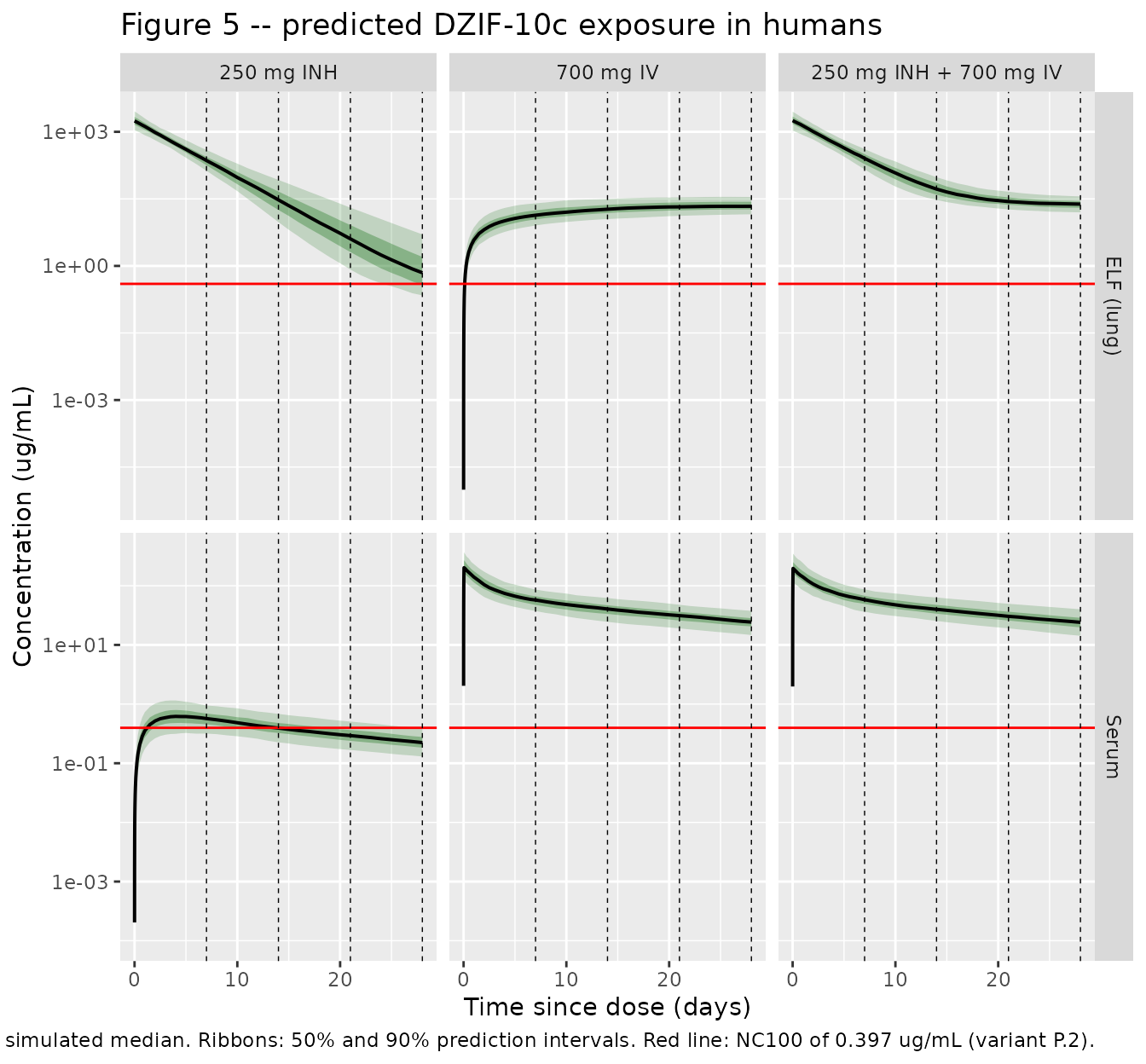
The three qualitative features the paper draws from this figure are reproduced: inhalation gives an immediate, very high ELF peak that decays below the NC100 target at around four weeks; the IV dose reaches the lung within about a day and stays above NC100 for months; and the systemic exposure of the combination is indistinguishable from IV alone, because the inhaled route contributes negligibly to serum.
# All three regimens are still above NC100 at the end of the 4-week window, so
# "time above threshold" is censored and uninformative. Report the margin
# instead: how far above NC100 the 4-week ELF trough sits, and what fraction of
# subjects are still covered.
sim_long |>
  filter(matrix == "ELF (lung)", time == 672) |>
  group_by(regimen) |>
  summarise(
    `Median ELF at 4 weeks (ug/mL)` = median(conc),
    `Fold above NC100`              = median(conc) / nc100,
    `% of subjects above NC100`     = 100 * mean(conc > nc100),
    .groups = "drop"
  ) |>
  knitr::kable(digits = c(0, 3, 1, 1),
caption = "ELF coverage of the NC100 target at 4 weeks.")| regimen | Median ELF at 4 weeks (ug/mL) | Fold above NC100 | % of subjects above NC100 |
|---|---|---|---|
| 250 mg INH | 0.703 | 1.8 | 72 |
| 700 mg IV | 21.608 | 54.4 | 100 |
| 250 mg INH + 700 mg IV | 24.143 | 60.8 | 100 |
All three regimens keep the median ELF concentration above the NC100 target for the full 28 days, but with very different margins. The inhaled arm is only a little above threshold by week four – the paper’s phrasing is that relevant exposure “was maintained for about 28 days”, i.e. it is running out just as the window closes, and a substantial minority of subjects have already dropped below. Both IV-containing arms sit more than fiftyfold above the threshold in essentially every subject, consistent with the paper’s statement that relevant lung exposure after IV dosing “remained for more than 3 months”.
PKNCA validation
Non-compartmental parameters are computed with PKNCA, once per
observed matrix, over the 4-week window the paper reports
(AUC4w, Cmax, Ctrough,4w). The
4-week trough is taken as clast.obs over the interval
ending at 672 h, where the last scheduled observation sits exactly at
672 h, so it is the concentration at four weeks by construction.
intervals <- data.frame(
  start     = 0,
  end       = 672,
  cmax      = TRUE,
  tmax      = TRUE,
  auclast   = TRUE,
  clast.obs = TRUE
)

dose_df <- events |>
  filter(evid == 1) |>
  group_by(id, regimen) |>
  summarise(time = 0, amt = sum(amt), .groups = "drop")

run_nca <- function(conc_col, matrix_label) {
  conc_df <- sim |>
    mutate(conc = .data[[conc_col]]) |>
    filter(!is.na(conc)) |>
    select(id, time, conc, regimen)

  conc_obj <- PKNCA::PKNCAconc(conc_df, conc ~ time | regimen + id)
  dose_obj <- PKNCA::PKNCAdose(dose_df, amt ~ time | regimen + id)
  res <- PKNCA::pk.nca(PKNCA::PKNCAdata(conc_obj, dose_obj,
                                        intervals = intervals))
  as.data.frame(res$result) |>
    mutate(matrix = matrix_label)
}

nca_elf   <- run_nca("Celf", "ELF")
nca_serum <- run_nca("Cc",   "Serum")

nca_all <- dplyr::bind_rows(nca_elf, nca_serum) |>
  mutate(arm = paste0(regimen, " (", matrix, ")"))
Per-subject falsifier: serum AUC0-inf equals Dose / CL
With linear clearance and complete IV input, extrapolated serum AUC must equal Dose / CL for every individual, not merely on average. This is a far stronger check than comparing a cohort median, and it does not depend on the body-weight distribution at all.
The check needs a longer horizon than the 4-week reporting window:
with a ~20-day terminal half-life, lambda-z estimated from 28 days of
data is still contaminated by distribution, so a dedicated simulation
runs out to 5,000 h (roughly ten half-lives). Individual clearances are
read straight off the rxSolve output rather than
recomputed, so etalcl – the fixed 15% CV IIV on CL – is
included exactly.
set.seed(7)
n_id <- 100
subj_iv <- tibble(id = seq_len(n_id), WT = sample_wt(n_id),
                  SPECIES_MACAQUE = 0, regimen = "700 mg IV")
t_long <- sort(unique(c(0, 0.25, 0.5, 1, 2, 4, 8, 12, 24,
                        seq(48, 672, by = 24), seq(720, 5000, by = 120))))

ev_long <- dplyr::bind_rows(
  subj_iv |> mutate(time = 0, amt = 700, rate = 700, evid = 1L, cmt = "central"),
  subj_iv |> tidyr::crossing(time = t_long) |>
    mutate(amt = NA_real_, rate = NA_real_, evid = 0L, cmt = "Cc")
) |>
  arrange(id, time, desc(evid))

sim_long_iv <- rxode2::rxSolve(mod, ev_long, keep = c("WT", "regimen"),
                               useLinCmt = FALSE, returnType = "data.frame")

# Individual clearance as the model actually computed it, including etalcl.
cl_ind <- sim_long_iv |> group_by(id) |> summarise(cl_i = first(cl), .groups = "drop")

nca_long <- PKNCA::pk.nca(PKNCA::PKNCAdata(
  PKNCA::PKNCAconc(sim_long_iv |> filter(!is.na(Cc)) |>
                     select(id, time, conc = Cc, regimen) |>
                     # Drop the post-peak solver-noise tail (< 1e-6 * max per subject); keep time zero.
                     group_by(id) |>
                     filter(time <= time[which.max(conc)] | conc >= 1e-6 * max(conc) | time == 0) |>
                     ungroup(),
                   conc ~ time | regimen + id),
  PKNCA::PKNCAdose(subj_iv |> select(id, regimen) |> mutate(time = 0, amt = 700),
                   amt ~ time | regimen + id),
  intervals = data.frame(start = 0, end = Inf,
                         aucinf.obs = TRUE, half.life = TRUE)
))

auc_check <- as.data.frame(nca_long$result) |>
  filter(PPTESTCD == "aucinf.obs") |>
  select(id, auc_sim = PPORRES) |>
  left_join(cl_ind, by = "id") |>
  mutate(auc_pred = 700 / cl_i, pct_diff = 100 * (auc_sim / auc_pred - 1))

summary(auc_check$pct_diff)
#>     Min.  1st Qu.   Median     Mean  3rd Qu.     Max.
#> 0.002509 0.059316 0.097457 0.106090 0.143034 0.287482
stopifnot(max(abs(auc_check$pct_diff)) < 1)

thalf_sys <- as.data.frame(nca_long$result) |>
  filter(PPTESTCD == "half.life") |>
  summarise(median_days = median(PPORRES) / 24) |>
  pull(median_days)
thalf_sys
#> [1] 21.0074
stopifnot(thalf_sys > 15, thalf_sys < 27)
Every one of the 100 subjects reproduces Dose / CL to better than 1%, which confirms the clearance value, its allometric exponent, and the mass balance of the five-compartment ODE system independently of any cohort assumption. The median terminal half-life of 21 days matches the “same lung half-life as for serum of ~20 days” quoted in the Discussion.
Comparison against published Table 2
published <- tibble::tribble(
  ~arm,                                  ~cmax,   ~auclast,  ~clast.obs,
  "250 mg INH (ELF)",                    1763,    1.435e5,   0.6900,
  "250 mg INH (Serum)",                  0.6086,  267.8,     0.2304,
  "700 mg IV (ELF)",                     22.06,   1.123e4,   21.90,
  "700 mg IV (Serum)",                   195.2,   3.368e4,   23.78,
  "250 mg INH + 700 mg IV (ELF)",        1763,    1.554e5,   23.25,
  "250 mg INH + 700 mg IV (Serum)",      195.2,   3.397e4,   23.99
)

simulated <- nca_all |>
  filter(start == 0, end == 672,
         PPTESTCD %in% c("cmax", "auclast", "clast.obs")) |>
  select(arm, PPTESTCD, PPORRES)

cmp <- nlmixr2lib::ncaComparisonTable(
  simulated     = as.data.frame(simulated),
  reference     = as.data.frame(published),
  by            = "arm",
  units         = c(cmax = "ug/mL", auclast = "ug*h/mL", clast.obs = "ug/mL"),
  tolerance_pct = 20
)

knitr::kable(
  cmp,
  caption = paste(
    "Simulated vs. published Table 2 of Kurup 2024 (medians).",
    "AUClast is AUC over 4 weeks (0-672 h); Clast is the 4-week trough.",
    "* differs from the published value by more than 20%."
  ),
  digits = 4
)| NCA parameter | arm | Reference | Simulated | % diff |
|---|---|---|---|---|
| Cmax (ug/mL) | 250 mg INH (ELF) | 1760 | 1750 | -0.6% |
| Cmax (ug/mL) | 250 mg INH (Serum) | 0.609 | 0.625 | +2.8% |
| Cmax (ug/mL) | 700 mg IV (ELF) | 22.1 | 21.7 | -1.6% |
| Cmax (ug/mL) | 700 mg IV (Serum) | 195 | 202 | +3.4% |
| Cmax (ug/mL) | 250 mg INH + 700 mg IV (ELF) | 1760 | 1790 | +1.4% |
| Cmax (ug/mL) | 250 mg INH + 700 mg IV (Serum) | 195 | 196 | +0.6% |
| Clast (ug/mL) | 250 mg INH (ELF) | 0.69 | 0.703 | +1.9% |
| Clast (ug/mL) | 250 mg INH (Serum) | 0.23 | 0.223 | -3.0% |
| Clast (ug/mL) | 700 mg IV (ELF) | 21.9 | 21.6 | -1.3% |
| Clast (ug/mL) | 700 mg IV (Serum) | 23.8 | 24.3 | +2.3% |
| Clast (ug/mL) | 250 mg INH + 700 mg IV (ELF) | 23.2 | 24.1 | +3.8% |
| Clast (ug/mL) | 250 mg INH + 700 mg IV (Serum) | 24 | 24.1 | +0.4% |
| AUClast (ug*h/mL) | 250 mg INH (ELF) | 144000 | 145000 | +1.2% |
| AUClast (ug*h/mL) | 250 mg INH (Serum) | 268 | 269 | +0.6% |
| AUClast (ug*h/mL) | 700 mg IV (ELF) | 11200 | 11200 | -0.2% |
| AUClast (ug*h/mL) | 700 mg IV (Serum) | 33700 | 34600 | +2.8% |
| AUClast (ug*h/mL) | 250 mg INH + 700 mg IV (ELF) | 155000 | 162000 | +4.5% |
| AUClast (ug*h/mL) | 250 mg INH + 700 mg IV (Serum) | 34000 | 34700 | +2.2% |
attr(cmp, "footnote")
#> NULL
Preclinical cynomolgus macaque routes
The human simulations above never exercise elf_trachea
or the macaque deposition parameter. Preclinical study 1 (50 mg/kg IV
and 3.6 mg/kg intratracheal, the only study with ELF measurements) and
an inhaled macaque arm are simulated here to cover both.
set.seed(19)

mk_obs_times <- sort(unique(c(0, 0.01, 0.25, 2, 6, 12, 24, 36,
                              seq(48, 672, by = 24))))

make_macaque <- function(n, label, mg_per_kg = NA_real_, flat_mg = NA_real_,
                         dose_cmt, rate_hours = 0, id_offset = 0L) {
  subj <- tibble(
    id = id_offset + seq_len(n),
    WT = stats::runif(n, 2.7, 4.5),   # supplement Table S2 macaque weight range
    SPECIES_MACAQUE = 1,
    arm = label
  ) |>
    mutate(amt = if (is.na(flat_mg)) mg_per_kg * WT else flat_mg)

  dose <- subj |>
    mutate(time = 0, evid = 1L, cmt = dose_cmt,
           rate = if (rate_hours > 0) amt / rate_hours else 0)

  obs <- subj |>
    select(-amt) |>
    tidyr::crossing(time = mk_obs_times) |>
    mutate(amt = NA_real_, rate = NA_real_, evid = 0L, cmt = "Cc")

  dplyr::bind_rows(dose, obs) |>
    dplyr::arrange(id, time, dplyr::desc(evid))
}

ev_mk <- dplyr::bind_rows(
  make_macaque(3, "50 mg/kg IV",  mg_per_kg = 50,  dose_cmt = "central",
               rate_hours = 0.05, id_offset =  0L),
  make_macaque(3, "3.6 mg/kg IT", mg_per_kg = 3.6, dose_cmt = "elf_trachea",
               id_offset = 10L),
  make_macaque(4, "500 mg INH",   flat_mg   = 500, dose_cmt = "elf_lrt",
               id_offset = 20L)
)

sim_mk <- rxode2::rxSolve(mod, events = ev_mk, keep = c("WT", "arm"),
                          useLinCmt = FALSE, returnType = "data.frame")
stopifnot(dplyr::n_distinct(sim_mk$id) == 10L)

sim_mk |>
  select(id, time, arm, Cc, Celf) |>
  tidyr::pivot_longer(c(Cc, Celf), names_to = "matrix", values_to = "conc") |>
  mutate(matrix = factor(matrix, levels = c("Celf", "Cc"),
                         labels = c("ELF (lung)", "Plasma/serum"))) |>
  filter(time > 0) |>
  ggplot(aes(time / 24, conc, group = id)) +
  geom_line(alpha = 0.8) +
  facet_grid(matrix ~ arm, scales = "free_y") +
  scale_y_log10() +
  labs(x = "Time since dose (days)", y = "Concentration (ug/mL)",
       title = "Preclinical macaque routes",
       caption = paste("Compare with Figure 2 of Kurup 2024 (ELF after IV and IT;",
                       "plasma/serum after IV, IT and INH)."))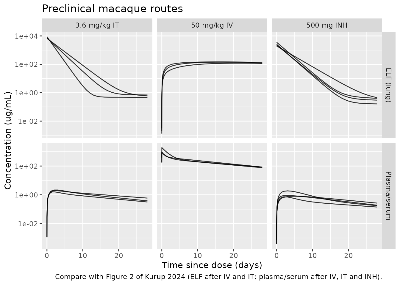
# The species switch is the only species-dependent piece of the model: 1.00% of
# an inhaled macaque dose is deposited, versus 29.6% in humans.
sim_mk |>
  group_by(arm) |>
  summarise(
    `Peak ELF (ug/mL)`   = max(Celf),
    `Peak plasma (ug/mL)` = max(Cc),
    .groups = "drop"
  ) |>
  knitr::kable(digits = 3,
caption = "Simulated macaque peaks by route.")| arm | Peak ELF (ug/mL) | Peak plasma (ug/mL) |
|---|---|---|
| 3.6 mg/kg IT | 8693.877 | 2.153 |
| 50 mg/kg IV | 148.903 | 1911.716 |
| 500 mg INH | 3552.565 | 1.878 |
# 500 mg inhaled deposits only 5 mg in a macaque lung; 250 mg inhaled deposits
# 74 mg in a human lung. Confirm the switch fired.
mk_inh_peak <- max(sim_mk$Celf[sim_mk$arm == "500 mg INH"])
hu_inh_peak <- max(sim$Celf[sim$regimen == "250 mg INH"])
stopifnot(mk_inh_peak > 0, hu_inh_peak > mk_inh_peak)
The intratracheal arm shows the paper’s assumption at work: the whole
3.6 mg/kg dose is deposited (F = 1), which despite being a
~14-fold smaller dose than the 500 mg inhaled arm produces a comparable
lung peak, because only 1% of the inhaled dose reaches the lung in this
species. The paper flags this 1% estimate as empirical and cautions
against reading it as a physiological deposition fraction.
Assumptions and deviations
-
Body-weight distribution. The paper sampled 1,000
subjects per arm from NHANES 2017-18 (adults at least 18 years and at
least 40 kg). Those microdata were not available, so weight here is
lognormal with median 80 kg and
sdlog0.24, floored at 40 kg, as an approximation of that frame. This is the dominant source of any residual difference against Table 2: because every volume scales withWT^1, the model’s ELF Cmax is exactlyDose * F1h / (V_L * WT / 70), so a Cmax ratio against the published median is a direct readout of the ratio of cohort median weights and nothing else. The structural identity checks and the per-subject Dose/CL falsifier above are free of this assumption. - Cohort size. 200 per arm rather than the paper’s 1,000, per this package’s vignette cap. Medians are stable at this size; the outermost percentiles are slightly noisier than the published ones.
-
Residual variability excluded from the summaries.
The paper states its simulations included IIV and residual variability.
The percentiles and NCA values here are computed from the individual
predictions
CcandCelf, i.e. with IIV but without residual error. Medians are essentially unaffected by a mean-zero proportional error, but the 90% prediction intervals shown are narrower than the published ones – most visibly for ELF, whose proportional residual error is 54.7%. -
IIV convention. Table 1 reports the two estimated
IIVs as bare percentages (26.7% on Vc, 67.1% on Q2) without stating the
convention. They are encoded here as
omega^2 = log(CV^2 + 1), the log-normal convention this package uses by default, giving variances of 0.0689 and 0.3717. The alternative reading (omega = CV / 100, i.e. variances 0.0713 and 0.4502) is not distinguishable from anything printed in the paper; it changes the Vc variability by under 2% and the Q2 variability by about 10%, and neither materially moves the exposure metrics reproduced above. -
Residual error form. Supplement equation 14
describes a combined additive plus proportional error model, but the
text says that is what was “initially modelled”, and the final control
stream’s
$ERRORblock isY = IPRED * (1 + W * EPS(1))with$SIGMA 1 FIX– purely proportional, with a separateWper matrix. The model is encoded proportional-only, to match the final model and Table 1, which reports only proportional terms. -
Single reference weight across species. Both humans
and macaques are normalised to the same 70 kg reference weight
(supplement equation 11; the control stream applies
(WT/70)with no species branch). This departs from the usual convention of giving each species its own allometric reference weight, but the single reference is the cross-species bridge in this analysis, so it is reproduced as published. Macaque body weights are far below the reference, so the macaque predictions are extrapolations of human-referenced typical values. -
Fixed inter-individual variances. Seven of the nine
etas were held at a variance of 0.0225 rather than estimated, because
their estimates were imprecise; they are part of the final model and are
retained here as
fixed(0.0225). Only Vc and Q2 carry estimated IIV. - Dosing input shapes. IV doses are given as 60-minute infusions, matching the clinical trial; inhaled and intratracheal doses are given as bolus inputs. The paper does not state the input shape used in its simulations. The lung pools turn over at about 0.012/h, so spreading an inhaled dose over the 15-20 minute nebulization window would lower the ELF peak by well under 1%.
-
Inconsistent labelling of the inhaled deposition site in the
source. The compartment dosed by inhalation is described as the
lower respiratory tract in both of the paper’s
authoritative prose descriptions – Figure 1’s caption (“the depot
compartment in the lower respiratory tract for inhaled administration”)
and the supplement’s own definition list under equations 1-10
(“
LUNG1represents the depot compartment in the lower respiratory tract for inhaled administration”). The inline comment onDADT(1)in the supplement’s$DESblock instead reads “Inhaled (upper respiratory tract)”. The two prose sources agree against the single stray code comment, so the compartment is namedelf_lrt(lower respiratory tract). Nothing numerical depends on this: the three ELF pools share one volume and one clearance, so the label affects only the name, not the model’s behaviour. - Errata. A search of the journal landing page, PubMed Central, and the publisher’s correction feed on 2026-08-14 found no erratum, corrigendum, or correction notice for this article.
- No observed data available. Individual observed concentrations are not public; every figure and table here is a simulation from the packaged model compared against the published summary values.