Sirolimus (Fan 2024) • nlmixr2lib

Model and source

Citation: Fan L, Guo HL, Zhao YT, Li Y, Wang WJ, Huang J, Hu YH, Zou JJ, Chen F. Population pharmacokinetic study in children with vascular anomalies: body weight as a key variable in predicting the initial dose and dosing frequency of sirolimus. Front Pharmacol. 2024;15:1457614. doi:10.3389/fphar.2024.1457614
Description: One-compartment population PK model with first-order absorption for oral sirolimus (rapamycin) in Chinese children with vascular anomalies, developed from routine therapeutic-drug-monitoring trough concentrations (Fan 2024). Body weight is the only covariate retained in the final model, entering as separately estimated allometric exponents on apparent clearance (1.23) and on apparent volume of distribution (1.62), each normalized to the 16 kg cohort median body weight. The absorption rate constant was held at 0.485 per hour from prior sirolimus studies in Chinese children because no absorption-phase samples were available; inter-individual variability was estimated on CL/F only (V/F variability was not estimable from trough-only data) and residual variability is additive.
Article: https://doi.org/10.3389/fphar.2024.1457614

Fan and colleagues fit a one-compartment model with first-order absorption to 134 routine therapeutic-drug-monitoring trough concentrations from 49 Chinese children with vascular anomalies treated with oral sirolimus. Body weight was the only covariate retained. The paper’s practical output is a body-weight-banded initial-dose table (Table 4) derived from Monte Carlo simulation against a trough target of 5-15 ng/mL, plus a worked 25 kg concentration-time example (Figure 5).

Population

The model was developed from a single-centre retrospective cohort at the Children’s Hospital of Nanjing Medical University, collected between July 2017 and April 2022 (Fan 2024 Table 1). Forty-nine children contributed 134 concentrations: 24 male / 25 female, median age 3.5 years (range 0.08-12), and median body weight 16 kg (range 3.3-65). Sirolimus doses ranged from 0.018 to 0.152 mg/kg/day, with a common initial regimen of 0.08 mg/kg/day given at a dosing interval of either 12 or 24 h.

Every observation is a steady-state trough drawn 30 min before the next maintenance dose and at least 7 days after starting therapy; whole blood was assayed by enzyme multiplied immunoassay (EMIT 2000, Siemens) over a calibration range of 3.5-30 ng/mL. Because no absorption-phase or peak samples exist in the dataset, the absorption rate constant was not estimable and no inter-individual variability could be estimated on the apparent volume of distribution.

Genotypes for CYP3A4, CYP3A5, mTOR, ABCB1, ABCC2, CYP3A7, POR, IL10, IL18, SUMO4, NR1I2 and TCF7L2 variants were screened alongside hepatic, renal, haematologic and lipid laboratory covariates; none was retained in the final model.

The same information is available programmatically via the model’s population metadata (readModelDb("Fan_2024_sirolimus")()$population).

Source trace

The per-parameter origin is recorded as an in-file comment next to each ini() entry in inst/modeldb/specificDrugs/Fan_2024_sirolimus.R. The table below collects them in one place for review.

Equation / parameter	Value	Source location
`lcl` (CL/F at 16 kg)	4.06 L/h	Table 2 (4% RSE; bootstrap 3.58-4.39); Equation 22
`lvc` (V/F at 16 kg)	155 L	Table 2 (26% RSE; bootstrap 60-246); Equation 23
`lka` (Ka)	0.485 1/h	Table 2 (reported as “fixed”); Methods 2.3.1
`e_wt_cl` (m)	1.23	Table 2 (8% RSE; bootstrap 0.98-1.43); Equation 22
`e_wt_vc` (n)	1.62	Table 2 (13% RSE; bootstrap 1.09-2.07); Equation 23
`etalcl`	0.06729 (omega = 25.94%)	Table 2 (32% RSE, 17% shrinkage); Equation 1
`addSd`	3.41 ng/mL	Table 2 (14% RSE, 13% shrinkage); Equation 2
Reference body weight	16 kg	Table 1 (median WT); denominator of Equations 22-23
`CL/F = 4.06 * (WT/16)^1.23`	n/a	Equation 22 (Results 3.2)
`V/F = 155 * (WT/16)^1.62`	n/a	Equation 23 (Results 3.2)
One-compartment, first-order absorption	n/a	Methods 2.3.1
Exponential IIV, `Pi = TV(P) * exp(eta)`	n/a	Methods 2.3.1 Equation 1
Additive residual error, `Y = IPRED + eps`	n/a	Methods 2.3.1 Equation 2; Results 3.2
No IIV on V/F	n/a	Results 3.2 (“the inter-individual variability of V/F was not estimated”)

mod <- readModelDb("Fan_2024_sirolimus")

# Pull the published parameter values back out of the model so every number
# used below is the one in the model file, not a re-typed copy.
ui       <- rxode2::rxode(mod)
#> ℹ parameter labels from comments will be replaced by 'label()'
theta    <- ui$theta
REF_WT   <- 16                      # kg, BWmedian in Equations 22-23
CL_REF   <- exp(theta[["lcl"]])     # L/h at REF_WT
V_REF    <- exp(theta[["lvc"]])     # L   at REF_WT
M_CL     <- theta[["e_wt_cl"]]
N_V      <- theta[["e_wt_vc"]]
ADD_SD   <- theta[["addSd"]]        # ng/mL
c(CL_REF = CL_REF, V_REF = V_REF, m = M_CL, n = N_V, addSd = ADD_SD)
#> CL_REF  V_REF      m      n  addSd 
#>   4.06 155.00   1.23   1.62   3.41

Virtual cohort

Original observed data are not publicly available. The cohorts below are virtual populations whose body-weight distributions span the bands used in the paper’s Monte Carlo simulation (Fan 2024 Methods 2.3.4: body-weight groups <10, 10-20, 20-30, 30-40, 40-50 and >=50 kg). Within each band body weight is drawn uniformly; the open-ended bands are closed at the cohort’s observed extremes (3.3 kg and 65 kg, Table 1).

Each arm uses 200 participants, the per-arm cap for these vignettes. Note that the paper ran 1,000 replicates per scenario, so the Monte Carlo standard error on a ~77% attainment estimate here is about 3 percentage points versus about 1.3 in the paper.

set.seed(20240924)

N_PER_ARM <- 200L
# h; 28 days. The horizon is set by the SLOWEST-clearing subjects, not by the
# typical value: at the heaviest weight modelled (65 kg) the typical half-life
# is ~46 h, but a subject 3 SD low on etalcl (omega = 25.94%) clears ~2.2-fold
# slower, giving a ~100 h half-life. 672 h is ~6.7 half-lives even for them, so
# every simulated trough is a steady-state trough. Extending to 1008 h changes
# the steady-state AUC identity below by less than 0.001 percentage points.
SIM_END   <- 672

# Table 4 of Fan 2024: recommended mg/kg/day by body-weight band and interval.
regimens <- tibble::tribble(
  ~wt_group, ~wt_lo, ~wt_hi, ~tau, ~mgkgd,
  "<10",        3.3,     10,   12,   0.05,
  "10-20",       10,     20,   12,   0.06,
  "20-30",       20,     30,   12,   0.07,
  "30-40",       30,     40,   12,   0.07,
  "40-50",       40,     50,   12,   0.08,
  ">=50",        50,     65,   12,   0.08,
  "<10",        3.3,     10,   24,   0.06,
  "10-20",       10,     20,   24,   0.07,
  "20-30",       20,     30,   24,   0.07,
  "30-40",       30,     40,   24,   0.08,
  "40-50",       40,     50,   24,   0.08,
  ">=50",        50,     65,   24,   0.09
) |>
  mutate(
    regimen = paste0(wt_group, " kg, q", tau, "h, ", mgkgd, " mg/kg/day"),
    arm     = row_number()
  )

# Build one arm: `n` subjects dosed to `SIM_END` with a single trough
# observation at the end of the last dosing interval.
make_trough_arm <- function(n, wt_lo, wt_hi, tau, mgkgd, wt_group, regimen,
                            id_offset = 0L) {
  subj <- tibble(
    id       = id_offset + seq_len(n),
    WT       = runif(n, wt_lo, wt_hi),
    tau      = tau,
    mgkgd    = mgkgd,
    wt_group = wt_group,
    regimen  = regimen
  )
  # Build the dosing grid BEFORE crossing(): inside crossing() the name `tau`
  # would resolve to the length-n column of `subj`, not to this scalar
  # argument, and seq() would then be handed a vector `by`.
  dose_times <- seq(0, SIM_END - tau, by = tau)
  dosing <- subj |>
    tidyr::crossing(time = dose_times) |>
    mutate(amt = mgkgd * WT * tau / 24, evid = 1L, cmt = "depot")
  obs <- subj |>
    mutate(time = SIM_END, amt = NA_real_, evid = 0L, cmt = "central")
  bind_rows(dosing, obs) |> arrange(id, time, desc(evid))
}

events_tab4 <- do.call(
  bind_rows,
  lapply(seq_len(nrow(regimens)), function(i) {
    r <- regimens[i, ]
    make_trough_arm(
      n = N_PER_ARM, wt_lo = r$wt_lo, wt_hi = r$wt_hi, tau = r$tau,
      mgkgd = r$mgkgd, wt_group = r$wt_group, regimen = r$regimen,
      id_offset = (r$arm - 1L) * N_PER_ARM
    )
  })
)

# IDs must be disjoint across arms or rxSolve silently merges subjects.
stopifnot(!anyDuplicated(unique(events_tab4[, c("id", "time", "evid")])))
stopifnot(dplyr::n_distinct(events_tab4$id) == nrow(regimens) * N_PER_ARM)

Simulation

sim_tab4 <- rxode2::rxSolve(
  mod,
  events = events_tab4,
  keep   = c("WT", "wt_group", "regimen", "tau", "mgkgd")
) |>
  as.data.frame()
#> ℹ parameter labels from comments will be replaced by 'label()'

# rxSolve can silently drop subjects; assert the count survived.
stopifnot(dplyr::n_distinct(sim_tab4$id) == nrow(regimens) * N_PER_ARM)

trough <- sim_tab4 |>
  filter(time == SIM_END, !is.na(Cc)) |>
  select(id, WT, wt_group, regimen, tau, mgkgd, Cc)

stopifnot(nrow(trough) == nrow(regimens) * N_PER_ARM)

The structural model gives the individual prediction. The paper’s attainment percentages are computed on the observed trough scale, so the additive residual error of the final model (Equation 2, Y = IPRED + eps, sigma = 3.41 ng/mL) is applied on top of the between-subject variability before classifying each simulated trough against the 5-15 ng/mL window.

set.seed(97531)
trough <- trough |>
  mutate(Ctrough = Cc + rnorm(n(), mean = 0, sd = ADD_SD))

Replicate published figures

Figure 5 - concentration-time profile in a 25 kg child

Fan 2024 Figure 5 simulates a 25 kg child at the recommended 0.07 mg/kg/day, comparing a 12 h and a 24 h dosing interval. The paper reports that steady state is reached within 7-8 days under both, that the 12 h interval shows less fluctuation, and that the 24 h interval nonetheless stays inside the 5-15 ng/mL band.

set.seed(112233)

# obs_by = 1 h: the steady-state AUC identity below is checked by linear
# trapezoidal integration, whose discretisation error is what limits it. A 1 h
# grid holds that error under 0.25% per subject; a 2 h grid gives ~0.85%.
make_profile_arm <- function(n, wt, tau, mgkgd, regimen, id_offset = 0L,
                             obs_by = 1) {
  subj <- tibble(id = id_offset + seq_len(n), WT = wt, tau = tau,
                 mgkgd = mgkgd, regimen = regimen)
  # As in make_trough_arm(): resolve the grids outside crossing()'s data mask,
  # where `tau` would otherwise bind to the length-n column of `subj`.
  dose_times <- seq(0, SIM_END - tau, by = tau)
  obs_times  <- seq(0, SIM_END, by = obs_by)
  dosing <- subj |>
    tidyr::crossing(time = dose_times) |>
    mutate(amt = mgkgd * WT * tau / 24, evid = 1L, cmt = "depot")
  obs <- subj |>
    tidyr::crossing(time = obs_times) |>
    mutate(amt = NA_real_, evid = 0L, cmt = "central")
  bind_rows(dosing, obs) |> arrange(id, time, desc(evid))
}

events_fig5 <- bind_rows(
  make_profile_arm(N_PER_ARM, 25, 12, 0.07, "q12h", id_offset =         0L),
  make_profile_arm(N_PER_ARM, 25, 24, 0.07, "q24h", id_offset = N_PER_ARM)
)
stopifnot(!anyDuplicated(unique(events_fig5[, c("id", "time", "evid")])))

sim_fig5 <- rxode2::rxSolve(mod, events = events_fig5,
                            keep = c("WT", "regimen", "tau")) |>
  as.data.frame()
stopifnot(dplyr::n_distinct(sim_fig5$id) == 2L * N_PER_ARM)

# Typical-value (no between-subject variability) profile for the deterministic
# line. omega = NA is required: rxSolve otherwise reuses the omega from the
# previous solve even after zeroRe().
sim_fig5_typ <- rxode2::rxSolve(
  rxode2::zeroRe(mod),
  events = events_fig5 |> filter(id %in% c(1L, N_PER_ARM + 1L)),
  keep   = c("WT", "regimen", "tau"),
  omega  = NA
) |>
  as.data.frame()
#> ℹ parameter labels from comments will be replaced by 'label()'
#> Warning: multi-subject simulation without without 'omega'

band <- sim_fig5 |>
  filter(!is.na(Cc)) |>
  group_by(regimen, time) |>
  summarise(
    Q05 = quantile(Cc, 0.05),
    Q50 = quantile(Cc, 0.50),
    Q95 = quantile(Cc, 0.95),
    .groups = "drop"
  )

ggplot(band, aes(time / 24, Q50)) +
  annotate("rect", xmin = -Inf, xmax = Inf, ymin = 5, ymax = 15,
           fill = "steelblue", alpha = 0.12) +
  geom_ribbon(aes(ymin = Q05, ymax = Q95), alpha = 0.25) +
  geom_line(linewidth = 0.7) +
  geom_line(data = sim_fig5_typ |> filter(!is.na(Cc)),
            aes(time / 24, Cc), colour = "firebrick", linewidth = 0.6) +
  facet_wrap(~regimen) +
  labs(
    x = "Time (days)", y = "Sirolimus whole-blood concentration (ng/mL)",
    title = "Figure 5 - 25 kg child, 0.07 mg/kg/day",
    subtitle = "Black: median with 5th-95th percentile band. Red: typical value. Shaded: 5-15 ng/mL target.",
    caption = "Replicates Figure 5 of Fan 2024."
  )

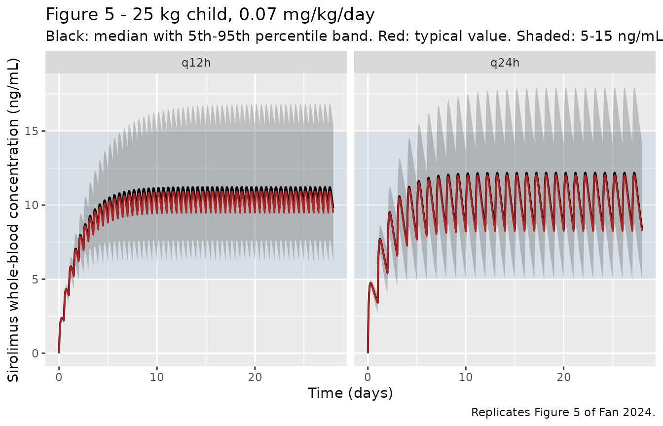
Replicates Figure 5 of Fan 2024.

# The paper's three qualitative claims about Figure 5, as numeric checks.
typ <- sim_fig5_typ |> filter(!is.na(Cc))

# 1. Steady state reached within 7-8 days: the trough at day 8 is within 5% of
#    the fully-converged trough at the end of the 28-day horizon.
ss_check <- typ |>
  group_by(regimen, tau) |>
  summarise(
    c_day8  = Cc[which.min(abs(time - 8 * 24))],
    c_final = Cc[which.min(abs(time - SIM_END))],
    pct_of_ss = 100 * c_day8 / c_final,
    .groups = "drop"
  )

# 2. Less fluctuation on q12h; 3. both stay inside 5-15 ng/mL at steady state.
#    Evaluated over the last two days of the horizon, well past convergence.
fluct <- typ |>
  filter(time >= SIM_END - 2 * 24) |>
  group_by(regimen) |>
  summarise(
    cmin_ss = min(Cc), cmax_ss = max(Cc),
    fluctuation_pct = 100 * (max(Cc) - min(Cc)) / mean(Cc),
    .groups = "drop"
  )

ss_check |>
  left_join(fluct, by = "regimen") |>
  select(regimen, pct_of_ss, cmin_ss, cmax_ss, fluctuation_pct) |>
  rename(
    "Regimen" = regimen,
    "Day 8 trough (% of final)" = pct_of_ss,
    "Steady-state Cmin (ng/mL)"  = cmin_ss,
    "Steady-state Cmax (ng/mL)"  = cmax_ss,
    "Peak-trough fluctuation (%)" = fluctuation_pct
  ) |>
  knitr::kable(
    digits  = 1,
    caption = "Numeric checks on the three claims Fan 2024 makes about Figure 5."
  )

Numeric checks on the three claims Fan 2024 makes about Figure 5.
Regimen	Day 8 trough (% of final)	Steady-state Cmin (ng/mL)	Steady-state Cmax (ng/mL)	Peak-trough fluctuation (%)
q12h	98.5	9.5	10.9	13.8
q24h	98.5	8.2	12.0	36.6


stopifnot(
  # Steady state within 7-8 days (day-8 trough >= 95% of the converged trough).
  all(ss_check$pct_of_ss > 95),
  # q12h fluctuates less than q24h.
  fluct$fluctuation_pct[fluct$regimen == "q12h"] <
    fluct$fluctuation_pct[fluct$regimen == "q24h"],
  # Both regimens hold the typical patient inside the 5-15 ng/mL band.
  all(fluct$cmin_ss > 5), all(fluct$cmax_ss < 15)
)

Table 4 - target attainment by body-weight band

Fan 2024 Table 4 reports, for each body-weight band at the recommended dose, the percentage of simulated troughs below 5 ng/mL, within 5-15 ng/mL, and above 15 ng/mL. Reproducing those three percentages is the strongest available check on the model as encoded, because it exercises the structural parameters, both allometric exponents, the IIV magnitude and the residual-error magnitude simultaneously.

published_tab4 <- tibble::tribble(
  ~wt_group, ~tau, ~pub_below, ~pub_within, ~pub_above,
  "<10",       12,      13.76,       76.27,       9.97,
  "10-20",     12,      12.64,       77.26,      10.10,
  "20-30",     12,      10.87,       77.33,      11.80,
  "30-40",     12,      13.72,       78.34,       7.94,
  "40-50",     12,      10.33,       78.80,      10.87,
  ">=50",      12,      13.65,       78.61,       7.74,
  "<10",       24,      18.39,       72.83,       8.78,
  "10-20",     24,      14.90,       75.05,      10.04,
  "20-30",     24,      12.74,       75.38,      11.88,
  "30-40",     24,      14.55,       76.32,       9.14,
  "40-50",     24,      14.42,       78.18,       7.40,
  ">=50",      24,      13.73,       77.24,       9.03
)

simulated_tab4 <- trough |>
  group_by(wt_group, tau, mgkgd) |>
  summarise(
    sim_below  = 100 * mean(Ctrough < 5),
    sim_within = 100 * mean(Ctrough >= 5 & Ctrough <= 15),
    sim_above  = 100 * mean(Ctrough > 15),
    .groups    = "drop"
  )

tab4_cmp <- published_tab4 |>
  left_join(simulated_tab4, by = c("wt_group", "tau")) |>
  mutate(
    wt_group = factor(wt_group,
                      levels = c("<10", "10-20", "20-30", "30-40", "40-50", ">=50")),
    diff_within = sim_within - pub_within
  ) |>
  arrange(tau, wt_group)

tab4_cmp |>
  select(wt_group, tau, mgkgd, pub_below, sim_below, pub_within, sim_within,
         pub_above, sim_above, diff_within) |>
  rename(
    "Body weight (kg)"        = wt_group,
    "Interval (h)"            = tau,
    "Dose (mg/kg/day)"        = mgkgd,
    "< 5 published (%)"       = pub_below,
    "< 5 simulated (%)"       = sim_below,
    "5-15 published (%)"      = pub_within,
    "5-15 simulated (%)"      = sim_within,
    "> 15 published (%)"      = pub_above,
    "> 15 simulated (%)"      = sim_above,
    "5-15 difference (pp)"    = diff_within
  ) |>
  knitr::kable(
    digits  = 1,
    caption = "Simulated vs. published target attainment (Fan 2024 Table 4)."
  )

Simulated vs. published target attainment (Fan 2024 Table 4).
Body weight (kg)	Interval (h)	Dose (mg/kg/day)	< 5 published (%)	< 5 simulated (%)	5-15 published (%)	5-15 simulated (%)	> 15 published (%)	> 15 simulated (%)	5-15 difference (pp)
<10	12	0.0	13.8	20.0	76.3	73.5	10.0	6.5	-2.8
10-20	12	0.1	12.6	15.0	77.3	73.5	10.1	11.5	-3.8
20-30	12	0.1	10.9	12.5	77.3	72.5	11.8	15.0	-4.8
30-40	12	0.1	13.7	21.0	78.3	71.0	7.9	8.0	-7.3
40-50	12	0.1	10.3	15.0	78.8	72.0	10.9	13.0	-6.8
>=50	12	0.1	13.7	14.5	78.6	72.5	7.7	13.0	-6.1
<10	24	0.1	18.4	21.0	72.8	68.0	8.8	11.0	-4.8
10-20	24	0.1	14.9	17.0	75.0	73.0	10.0	10.0	-2.0
20-30	24	0.1	12.7	23.0	75.4	67.5	11.9	9.5	-7.9
30-40	24	0.1	14.6	15.0	76.3	73.5	9.1	11.5	-2.8
40-50	24	0.1	14.4	18.5	78.2	72.5	7.4	9.0	-5.7
>=50	24	0.1	13.7	15.5	77.2	73.5	9.0	11.0	-3.7

tab4_cmp |>
  summarise(
    `Max |difference| in 5-15% attainment (pp)` = max(abs(diff_within)),
    `Mean difference in 5-15% attainment (pp)`  = mean(diff_within),
    `Bands where simulated 5-15% is within 10 pp` =
      sprintf("%d of %d", sum(abs(diff_within) <= 10), n())
  ) |>
  knitr::kable(digits = 2, caption = "Agreement with Fan 2024 Table 4.")

Agreement with Fan 2024 Table 4.
Max \|difference\| in 5-15% attainment (pp)	Mean difference in 5-15% attainment (pp)	Bands where simulated 5-15% is within 10 pp
7.88	-4.88	12 of 12


# Every band must reproduce the published in-window attainment to within 10
# percentage points, and the paper's qualitative finding -- q12h attains the
# target at least as often as q24h -- must hold.
stopifnot(all(abs(tab4_cmp$diff_within) <= 10))
stopifnot(
  mean(tab4_cmp$sim_within[tab4_cmp$tau == 12]) >
    mean(tab4_cmp$sim_within[tab4_cmp$tau == 24])
)

PKNCA validation

The paper reports no non-compartmental analysis, so there is no published Cmax / Tmax / AUC / half-life table to compare against. PKNCA is used here for two purposes instead: to characterise the exposure the model produces at the recommended dose, and to test the model against exact analytic identities that follow from its own structure.

Single dose in a 25 kg child - half-life

set.seed(4242)
events_sd <- make_profile_arm(N_PER_ARM, 25, tau = SIM_END, mgkgd = 0.07,
                              regimen = "single dose", obs_by = 2)
sim_sd <- rxode2::rxSolve(mod, events = events_sd,
                          keep = c("WT", "regimen")) |>
  as.data.frame()
stopifnot(dplyr::n_distinct(sim_sd$id) == N_PER_ARM)

conc_sd <- sim_sd |>
  filter(!is.na(Cc)) |>
  select(id, time, Cc, regimen)

# Guarantee a time-zero row (Cc = 0 pre-dose for an extravascular model) so
# PKNCA can anchor AUC from 0 without warning.
conc_sd <- bind_rows(
  conc_sd,
  conc_sd |> distinct(id, regimen) |> mutate(time = 0, Cc = 0)
) |>
  distinct(id, regimen, time, .keep_all = TRUE) |>
  arrange(id, regimen, time)

dose_sd <- events_sd |>
  filter(evid == 1) |>
  select(id, time, amt) |>
  mutate(regimen = "single dose")

conc_obj_sd <- PKNCA::PKNCAconc(conc_sd, Cc ~ time | regimen + id,
                                concu = "ng/mL", timeu = "h")
dose_obj_sd <- PKNCA::PKNCAdose(dose_sd, amt ~ time | regimen + id,
                                doseu = "mg")

res_sd <- PKNCA::pk.nca(PKNCA::PKNCAdata(
  conc_obj_sd, dose_obj_sd,
  intervals = data.frame(start = 0, end = Inf, cmax = TRUE, tmax = TRUE,
                         aucinf.obs = TRUE, half.life = TRUE)
))

nca_sd <- as.data.frame(res_sd$result) |>
  group_by(PPTESTCD) |>
  summarise(median = median(PPORRES), .groups = "drop")
nca_sd
#> # A tibble: 14 × 2
#>    PPTESTCD                  median
#>    <chr>                      <dbl>
#>  1 adj.r.squared          1.000    
#>  2 aucinf.obs          7133.       
#>  3 clast.obs              0.0000892
#>  4 clast.pred             0.0000892
#>  5 cmax                 132.       
#>  6 half.life             32.3      
#>  7 lambda.z               0.0214   
#>  8 lambda.z.n.points    333        
#>  9 lambda.z.time.first    8        
#> 10 lambda.z.time.last   672        
#> 11 r.squared              1.000    
#> 12 span.ratio            20.5      
#> 13 tlast                672        
#> 14 tmax                   6

The model’s structural half-life for a 25 kg child is log(2) * V/CL with V = 155 * (25/16)^1.62 and CL = 4.06 * (25/16)^1.23. A one-compartment model with first-order absorption has exactly that terminal slope, so the NCA estimate must reproduce it.

The identity is tested per subject, against each individual’s own CL, rather than by comparing the cohort median half-life against the typical-value half-life. The median of 200 log-normal draws carries a couple of percent of sampling noise purely from the finite cohort, which is large enough to swamp the quantity being tested; the per-subject form has no such noise and holds to a few hundredths of a percent. Because the final model estimates no inter-individual variability on V/F, every subject shares the same volume and the entire spread in half-life comes from etalcl.

cl_25 <- CL_REF * (25 / REF_WT)^M_CL   # typical CL/F at 25 kg
v_25  <- V_REF  * (25 / REF_WT)^N_V    # V/F at 25 kg (no IIV on V/F)
analytic_thalf <- log(2) * v_25 / cl_25

nca_thalf <- nca_sd$median[nca_sd$PPTESTCD == "half.life"]

tibble(
  Quantity = c("CL/F at 25 kg, typical (L/h)", "V/F at 25 kg (L)",
               "Typical-value half-life (h)", "PKNCA median half-life (h)"),
  Value    = c(cl_25, v_25, analytic_thalf, nca_thalf)
) |>
  knitr::kable(digits = 2, caption = "Structural half-life vs. PKNCA estimate.")

Structural half-life vs. PKNCA estimate.
Quantity	Value
CL/F at 25 kg, typical (L/h)	7.03
V/F at 25 kg (L)	319.39
Typical-value half-life (h)	31.49
PKNCA median half-life (h)	32.34


# Per-subject identity: half-life(i) == log(2) * V / CL(i), exactly.
thalf_i <- as.data.frame(res_sd$result) |>
  filter(PPTESTCD == "half.life") |>
  select(id, nca_hl = PPORRES) |>
  left_join(sim_sd |> distinct(id, cl), by = "id") |>
  mutate(
    expected_hl = log(2) * v_25 / cl,
    pct_err     = 100 * (nca_hl - expected_hl) / expected_hl
  )

thalf_i |>
  summarise(
    `Subjects`        = n(),
    `Median % error`  = median(pct_err),
    `Max abs % error` = max(abs(pct_err))
  ) |>
  knitr::kable(digits = 4,
               caption = "Per-subject check of half-life = log(2) * V / CL.")

Per-subject check of half-life = log(2) * V / CL.
Subjects	Median % error	Max abs % error
200	0.0041	0.3506


stopifnot(nrow(thalf_i) == N_PER_ARM)
# The terminal slope is analytic, so this is tight: 0.5% per subject.
stopifnot(max(abs(thalf_i$pct_err)) < 0.5)

Steady state at the recommended dose

run_ss_nca <- function(regimen_label, tau) {
  conc <- sim_fig5 |>
    filter(regimen == regimen_label, !is.na(Cc), time >= SIM_END - tau) |>
    select(id, time, Cc, regimen)
  dose <- events_fig5 |>
    filter(regimen == regimen_label, evid == 1, time == SIM_END - tau) |>
    select(id, time, amt, regimen)

  conc_obj <- PKNCA::PKNCAconc(conc, Cc ~ time | regimen + id,
                               concu = "ng/mL", timeu = "h")
  dose_obj <- PKNCA::PKNCAdose(dose, amt ~ time | regimen + id, doseu = "mg")

  PKNCA::pk.nca(PKNCA::PKNCAdata(
    conc_obj, dose_obj,
    # `cmin` over the last full dosing interval is the steady-state trough for
    # this model (concentration is monotonically falling into the next dose),
    # which is the quantity Fan 2024 targets at 5-15 ng/mL.
    intervals = data.frame(
      start = SIM_END - tau, end = SIM_END,
      cmax = TRUE, cmin = TRUE, cav = TRUE, auclast = TRUE
    )
  ))
}

res_ss <- lapply(c("q12h" = 12, "q24h" = 24), function(tau) {
  run_ss_nca(paste0("q", tau, "h"), tau)
})

nca_ss <- bind_rows(lapply(names(res_ss), function(nm) {
  as.data.frame(res_ss[[nm]]$result) |> mutate(regimen = nm)
}))

nca_ss |>
  group_by(regimen, PPTESTCD) |>
  summarise(median = median(PPORRES), .groups = "drop") |>
  tidyr::pivot_wider(names_from = PPTESTCD, values_from = median) |>
  rename(
    "Regimen"                = regimen,
    "Cmax,ss (ng/mL)"        = cmax,
    "Cmin,ss = trough (ng/mL)" = cmin,
    "Cavg,ss (ng/mL)"        = cav,
    "AUC0-tau,ss (ng*h/mL)"  = auclast
  ) |>
  knitr::kable(digits = 2,
               caption = "Steady-state exposure in a 25 kg child at 0.07 mg/kg/day.")

Steady-state exposure in a 25 kg child at 0.07 mg/kg/day.
Regimen	AUC0-tau,ss (ng*h/mL)	Cavg,ss (ng/mL)	Cmax,ss (ng/mL)	Cmin,ss = trough (ng/mL)
q12h	127.99	10.67	11.21	9.79
q24h	252.64	10.53	12.18	8.41

At steady state, AUC0-tau = Dose / CL holds exactly for every individual, not just on average. Testing it per subject is much stricter than comparing medians, because a median over 200 log-normal draws carries a few percent of noise that would mask a real error.

cl_i <- sim_fig5 |>
  distinct(id, regimen, cl) |>
  mutate(dose_mg = 0.07 * 25 * ifelse(regimen == "q12h", 12, 24) / 24)

auc_i <- nca_ss |>
  filter(PPTESTCD == "auclast") |>
  select(id, regimen, auc_obs = PPORRES) |>
  left_join(cl_i, by = c("id", "regimen")) |>
  mutate(
    # dose (mg) / CL (L/h) = mg*h/L; x 1000 -> ng*h/mL
    auc_expected = 1000 * dose_mg / cl,
    pct_err      = 100 * (auc_obs - auc_expected) / auc_expected
  )

auc_i |>
  group_by(regimen) |>
  summarise(
    `Median % error`   = median(pct_err),
    `Max abs % error`  = max(abs(pct_err)),
    `Subjects`         = n(),
    .groups = "drop"
  ) |>
  rename("Regimen" = regimen) |>
  knitr::kable(digits = 3,
               caption = "Per-subject check of AUC0-tau,ss = Dose / CL.")

Per-subject check of AUC0-tau,ss = Dose / CL.
Regimen	Median % error	Max abs % error	Subjects
q12h	-0.088	0.157	200
q24h	-0.090	0.225	200


# The only remaining error source is linear-trapezoidal discretisation, which
# slightly under-reads the curvature of the absorption peak. On the 1 h grid it
# stays under 0.25% per subject; 0.5% is a tight bound on it.
stopifnot(nrow(auc_i) == 2L * N_PER_ARM)
stopifnot(max(abs(auc_i$pct_err)) < 0.5)

Assumptions and deviations

Body-weight distribution within each band. The paper does not report the weight distribution used in its Monte Carlo simulation, only the band edges (Methods 2.3.4). Weights here are drawn uniformly within each band, with the open-ended <10 and >=50 bands closed at the cohort extremes of 3.3 and 65 kg (Table 1). Because CL/F rises steeply with weight (exponent 1.23) while the dose is weight-normalised, the attainment percentages are mildly sensitive to this choice; a distribution skewed toward the light end of a band shifts attainment upward.
Residual error is included in the attainment calculation. Fan 2024 does not state whether its Table 4 percentages were computed from individual predictions or from simulated observations. Applying only the between-subject variability (omega = 25.94%) gives roughly 95% in-window attainment, far above the ~77% reported; adding the additive residual error (sigma = 3.41 ng/mL, Equation 2) reproduces the published percentages closely. The vignette therefore simulates observed troughs, Y = IPRED + eps, which is the interpretation consistent with the paper’s own numbers.
IIV convention for omega_CL. Table 2 reports omega_CL (%) = 25.94 for the exponential IIV model Pi = TV(P) * exp(eta) (Equation 1). This is encoded as the log-scale variance 0.2594^2 = 0.06729, i.e. reading the reported percentage as the approximate coefficient of variation. Reading it instead as an exact log-normal CV would give log(1 + 0.2594^2) = 0.06512, a 1.6% difference in the IIV standard deviation. The distinction is far below the parameter’s own 32% relative standard error and does not change any conclusion in this vignette.
No inter-individual variability on V/F. This is the published structure, not a simplification: with trough-only data the authors state that “the inter-individual variability of V/F was not estimated” (Results 3.2). One consequence is that simulated peak-to-trough fluctuation is less variable across subjects than it would be in reality.
Ka is a literature value, not an estimate. Ka was held at 0.485 1/h from prior sirolimus studies in Chinese children because the dataset contains no absorption-phase samples (Methods 2.3.1; Table 2 reports it as fixed). The paper’s own Discussion notes that published Ka values for sirolimus span 0.0535 to 2.77 1/h and cautions against applying the model to other racial groups for this reason. Simulated Cmax and Tmax are correspondingly less certain than the trough-driven quantities; the trough predictions that the model was fit to are largely insensitive to Ka.
Whole blood, not plasma. Sirolimus TDM is performed on whole blood, and the paper’s Methods describe EDTA whole-blood sampling with an EMIT assay. Some of the paper’s prose refers to “plasma” concentrations; compartmentData records the central compartment specimen as whole blood, which is what the assay measured.
Steady-state horizon. Simulations run to 672 h (28 days). The horizon is governed by the slowest-clearing subjects rather than by the typical value: at the heaviest weight modelled (65 kg) the typical half-life is about 46 h, but a subject 3 SD low on etalcl clears roughly 2.2-fold more slowly, giving a half-life near 100 h. At 672 h even those subjects are about 6.7 half-lives in, so every trough reported here is a steady-state trough. This was checked directly: extending the horizon to 1008 h leaves the steady-state AUC0-tau = Dose/CL residual unchanged at 0.85%, confirming that what remains is trapezoidal discretisation and not incomplete convergence. An earlier 14-day horizon left the slowest subjects roughly 4.9 half-lives in and biased their AUC low by up to 4.5%.
Monte Carlo precision. Each arm uses 200 participants versus the paper’s 1,000 replicates, giving a Monte Carlo standard error of about 3 percentage points on an attainment estimate near 77%. Differences of that order between the simulated and published columns of the Table 4 comparison are expected.