Vildagliptin (Landersdorfer 2012)
Source:vignettes/articles/Landersdorfer_2012_vildagliptin.Rmd
Landersdorfer_2012_vildagliptin.RmdModel and source
- Citation: Landersdorfer CB, He YL, Jusko WJ. Mechanism-based population pharmacokinetic modelling in diabetes: vildagliptin as a tight binding inhibitor and substrate of dipeptidyl peptidase IV. Br J Clin Pharmacol. 2012;73(3):391-401. doi:10.1111/j.1365-2125.2011.04108.x
- Description: Mechanism-based population PK plus DPP-4 activity model for vildagliptin in patients with type 2 diabetes. Target-mediated drug disposition with capacity-limited slow-tight binding of vildagliptin to DPP-4 in plasma and tissue and partial hydrolysis of vildagliptin by DPP-4.
- Article: Br J Clin Pharmacol 2012;73(3):391-401
Landersdorfer et al. developed a mechanism-based population PK / DPP-4 activity model for vildagliptin in patients with type 2 diabetes. The model captures slight (over-)dose-proportional pharmacokinetics by encoding target-mediated drug disposition: vildagliptin binds DPP-4 in plasma and in tissue with slow tight binding kinetics, and a fraction of the bound drug is hydrolysed by DPP-4 to an inactive metabolite (k_deg). The companion paper (Landersdorfer 2012, ref [9] of the source) extends this PK / DPP-4 module with active GLP-1, glucose, and insulin sub-models; only the PK / DPP-4 module is packaged here.
Population
The fit population was 13 patients with type 2 diabetes (mean age 53.5 years, range 37-64; weight 91 kg mean, range 65-116; height 166 cm mean, range 148-183; 6 male / 7 female). Subjects had diabetes for at least 3 months and washed out of hypoglycaemic drugs for up to 4 weeks before dosing. The randomized, placebo-controlled, double-blind, four-way crossover study administered 10, 25, and 100 mg vildagliptin and placebo orally twice daily for 28 days each, with PK sampling on day 28 of each period (Landersdorfer 2012 Methods section “Study participants” and section “Study design and drug administration”; the demographic numbers above are summarised in Results, p. 393).
Bioavailability F was fixed at 77.2 % from a separate intravenous-dose study in healthy volunteers (He YL et al. 2007, ref [6] of the source paper).
The same information is available programmatically via
readModelDb("Landersdorfer_2012_vildagliptin")()$meta$population.
Source trace
Every model equation and population parameter is annotated inline in
inst/modeldb/specificDrugs/Landersdorfer_2012_vildagliptin.R.
The table below collects the full provenance for review.
| Equation / parameter | Value | Source location |
|---|---|---|
d/dt(depot) = -k_a1 * A_G1 |
– | Methods section “Structural models”, Eq for A_G1 |
d/dt(transit1) = k_a1 * A_G1 - k_a2 * A_G2 |
– | Methods section “Structural models”, Eq for A_G2 |
d/dt(central) = k_a2 * A_G2 - (CL + CL_ic)/V_C * A_C + CL_ic/V_P * A_P - V_maxC + k_off * DR_C |
– | Methods section “Structural models”, Eq for A_C |
d/dt(peripheral1) = CL_ic/V_C * A_C - CL_ic/V_P * A_P - V_maxP + k_off * DR_P |
– | Methods section “Structural models”, Eq for A_P |
d/dt(complex) = V_maxC - (k_off + k_deg) * DR_C |
– | Methods section “Structural models”, Eq for DR_C |
d/dt(complex_peripheral) = V_maxP - (k_off + k_deg) * DR_P |
– | Methods section “Structural models”, Eq for DR_P |
V_maxC = k_2 * (A_C / V_C) * (R_maxC - DR_C) / (K_d + A_C / V_C) |
– | Methods section “Structural models”, V_maxC Eq |
V_maxP = k_2 * (A_P / V_P) * (R_maxP - DR_P) / (K_d + A_P / V_P) |
– | Methods section “Structural models”, V_maxP Eq |
DPP4 activity = cf1 * (R_maxC - DR_C) |
– | Methods section “Structural models”, DPP-4 activity output Eq |
CL non-saturable clearance |
36.4 L/h | Table 1 (BSV 25%, SE 9%) |
V_C central volume |
22.2 L | Table 1 (BSV 37%, SE 11%) |
V_P peripheral volume |
97.3 L | Table 1 (BSV 37%, SE 13%) |
CL_ic inter-compartmental clearance |
40.1 L/h | Table 1 (BSV 34%, SE 11%) |
k_a1 first absorption rate |
1.26 /h | Table 1 (BSV 46%, SE 15%) |
k_a2 second absorption rate |
1.05 /h | Table 1 (BSV 14%, SE 4%) |
F bioavailability (fixed) |
0.772 | Table 1 footnote * (fixed from co-modelling with i.v. He 2007 data) |
K_d equilibrium dissociation constant |
71.9 nmol/L | Table 1 (BSV 54%, SE 16%) |
k_2 weak -> high-affinity complex rate |
23.4 /h | Table 1 (BSV 70%, SE 22%) |
k_off dissociation rate |
0.612 /h | Table 1 (BSV 94%, SE 27%) |
k_deg hydrolysis-by-DPP-4 rate |
0.110 /h | Table 1 (BSV 81%, SE 26%) |
R_maxC DPP-4 amount in central |
5.0 nmol | Table 1 (BSV 12%, SE 4%) |
R_maxP DPP-4 amount in peripheral |
13.0 umol = 13000 nmol | Table 1 (BSV 64%, SE 23%) |
cf1 activity conversion factor |
2.80 (mU/mL/min)/nmol | Table 1 (BSV 17%, SE 5%) |
CV_Vilda proportional residual |
48.7 % | Table 1 |
SD_Vilda additive residual |
0.99 ng/mL | Table 1 |
CV_DPP-4 proportional residual |
19.6 % | Table 1 |
SD_DPP-4 additive residual |
0.061 mU/mL/min | Table 1 |
Units check
Amounts in the model are nmol; volumes are L; so the internal
concentration A_C / V_C is nmol/L = nM. The bioanalytical
readout is ng/mL, which equals nM * MW_vildagliptin / 1000
(MW = 303.40 g/mol; PubChem CID 6918537). The binding-rate equation
V_maxC = k_2 * C * (R_max - DR) / (K_d + C) has units
(1/h) * (nmol/L) * (nmol) / (nmol/L) = nmol/h, matching
d/dt(complex). Dose-unit conversion mg -> nmol is folded
into f(depot) so the user passes amt in mg.
Virtual cohort
The original study is small (13 subjects, day-28 sampling on each of three dose periods) and the per-subject observations are not redistributed. We build three matched virtual cohorts at the published demographics, one per dose level, and run BID dosing to steady state before sampling the final dosing interval.
set.seed(20260615)

# Dosing schedule: BID for 7 days (14 doses), then a dense observation grid
# over the next 12 h (one BID dosing interval at steady state).
n_per_dose <- 40L
dose_times <- seq(0, by = 12, length.out = 14)
sample_window <- 12 * 13                                # = 156 h, start of last interval
obs_pre  <- seq(0, sample_window, by = 12)              # trough samples before SS
obs_post <- seq(sample_window, sample_window + 12, by = 0.25)
obs_times <- sort(unique(c(obs_pre, obs_post)))

make_cohort <- function(n, dose_mg, treatment, id_offset = 0L) {
  ids <- id_offset + seq_len(n)
  dosing <- tidyr::expand_grid(id = ids, time = dose_times) |>
    dplyr::mutate(
      amt       = dose_mg,
      evid      = 1L,
      cmt       = "depot",
      treatment = treatment
    )
  obs <- tidyr::expand_grid(id = ids, time = obs_times) |>
    dplyr::mutate(
      amt       = 0,
      evid      = 0L,
      cmt       = "Cc",
      treatment = treatment
    )
  dplyr::bind_rows(dosing, obs) |>
    dplyr::arrange(id, time, dplyr::desc(evid))
}

events <- dplyr::bind_rows(
  make_cohort(n_per_dose, dose_mg =  10, treatment =  "10 mg", id_offset =                 0L),
  make_cohort(n_per_dose, dose_mg =  25, treatment =  "25 mg", id_offset =       n_per_dose),
  make_cohort(n_per_dose, dose_mg = 100, treatment = "100 mg", id_offset = 2L * n_per_dose)
)
stopifnot(!anyDuplicated(unique(events[, c("id", "time", "evid")])))
Simulation
mod <- readModelDb("Landersdorfer_2012_vildagliptin")
sim <- rxode2::rxSolve(mod, events = events,
                       keep = c("treatment"),
                       returnType = "data.frame")
#> ℹ parameter labels from comments will be replaced by 'label()'
For the deterministic typical-value replication used to drive PKNCA below, we also simulate with the random effects zeroed out.
mod_typical <- rxode2::zeroRe(mod)
#> ℹ parameter labels from comments will be replaced by 'label()'
sim_typical <- rxode2::rxSolve(mod_typical, events = events,
                               keep = c("treatment"),
                               returnType = "data.frame")
#> ℹ omega/sigma items treated as zero: 'etalka1', 'etalka2', 'etalcl', 'etalvc', 'etalvp', 'etalq', 'etalkd', 'etalk2', 'etalkoff', 'etalkdeg', 'etalrmaxc', 'etalrmaxp', 'etalcf1'
#> Warning: multi-subject simulation without without 'omega'
Replicate published figures
Visual predictive checks at steady state (day 7, treated as a steady-state proxy for the paper’s day 28 – by day 7 the slowest of the binding rate constants k_deg = 0.110 /h has cycled through > 27 half-lives, so the system is well at steady state). Time on the x-axis is hours after the morning dose on the last day.
sim_plot <- sim |>
  dplyr::filter(time >= sample_window) |>
  dplyr::mutate(
    t_after_dose = time - sample_window,
    treatment    = factor(treatment, levels = c("10 mg", "25 mg", "100 mg"))
  )

vpc_conc <- sim_plot |>
  dplyr::group_by(treatment, t_after_dose) |>
  dplyr::summarise(
    Q05 = stats::quantile(Cc, 0.10, na.rm = TRUE),
    Q50 = stats::quantile(Cc, 0.50, na.rm = TRUE),
    Q95 = stats::quantile(Cc, 0.90, na.rm = TRUE),
    .groups = "drop"
  )

ggplot(vpc_conc, aes(x = t_after_dose, y = Q50)) +
  geom_ribbon(aes(ymin = Q05, ymax = Q95), alpha = 0.25, fill = "steelblue") +
  geom_line(colour = "steelblue4", linewidth = 0.8) +
  facet_wrap(~ treatment, scales = "free_y") +
  labs(
    x = "Time after morning dose (h)",
    y = "Vildagliptin concentration (ng/mL)",
    title = "Figure 2 - VPC of vildagliptin plasma concentrations by dose",
    caption = "Replicates Figure 2A-C of Landersdorfer 2012: median + 80% prediction interval."
  ) +
  theme_minimal()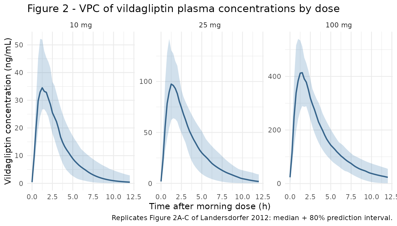
vpc_dpp4 <- sim_plot |>
  dplyr::group_by(treatment, t_after_dose) |>
  dplyr::summarise(
    Q05 = stats::quantile(DPP4, 0.10, na.rm = TRUE),
    Q50 = stats::quantile(DPP4, 0.50, na.rm = TRUE),
    Q95 = stats::quantile(DPP4, 0.90, na.rm = TRUE),
    .groups = "drop"
  )

ggplot(vpc_dpp4, aes(x = t_after_dose, y = Q50)) +
  geom_ribbon(aes(ymin = Q05, ymax = Q95), alpha = 0.25, fill = "tomato") +
  geom_line(colour = "tomato4", linewidth = 0.8) +
  facet_wrap(~ treatment) +
  labs(
    x = "Time after morning dose (h)",
    y = "DPP-4 activity (mU/mL/min)",
    title = "Figure 3 - VPC of DPP-4 activity by dose",
    caption = paste(
      "Replicates Figure 3 of Landersdorfer 2012.",
      "Baseline cf1 * R_maxC = 2.80 * 5.0 = 14.0 mU/mL/min."
    )
  ) +
  theme_minimal()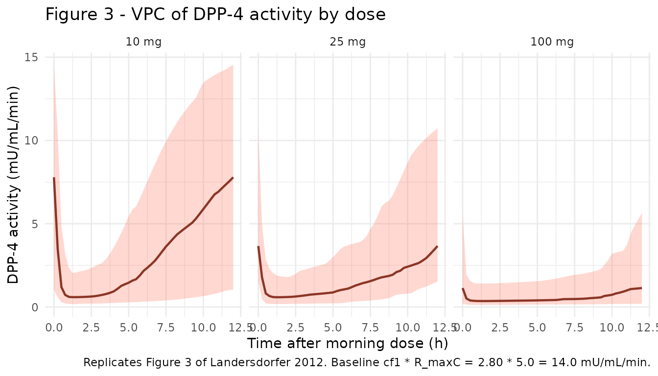
# Replicates Figure 4 of Landersdorfer 2012: mechanistic model components vs
# time at the 100 mg dose. We use the typical-value simulation and look at
# the same final-interval window.
mech <- sim_typical |>
  dplyr::filter(treatment == "100 mg", time >= sample_window) |>
  dplyr::mutate(t_after_dose = time - sample_window) |>
  dplyr::select(t_after_dose, Cc, DPP4, peripheral1, complex, complex_peripheral)

mech_long <- mech |>
  tidyr::pivot_longer(c(Cc, DPP4, peripheral1, complex, complex_peripheral),
                      names_to = "component", values_to = "value") |>
  dplyr::mutate(
    component = dplyr::recode(component,
      Cc                 = "Vildagliptin central (ng/mL)",
      DPP4               = "DPP-4 activity central (mU/mL/min)",
      peripheral1        = "Vildagliptin peripheral (nmol)",
      complex            = "Vilda-DPP4 complex central (nmol)",
      complex_peripheral = "Vilda-DPP4 complex peripheral (nmol)"
    )
  )

ggplot(mech_long, aes(x = t_after_dose, y = value)) +
  geom_line(linewidth = 0.7, colour = "grey20") +
  facet_wrap(~ component, scales = "free_y") +
  labs(
    x = "Time after morning dose (h)",
    y = NULL,
    title = "Figure 4 - mechanistic components at 100 mg (typical individual)",
    caption = "Replicates the model-component panel of Landersdorfer 2012 Figure 4."
  ) +
  theme_minimal(base_size = 9)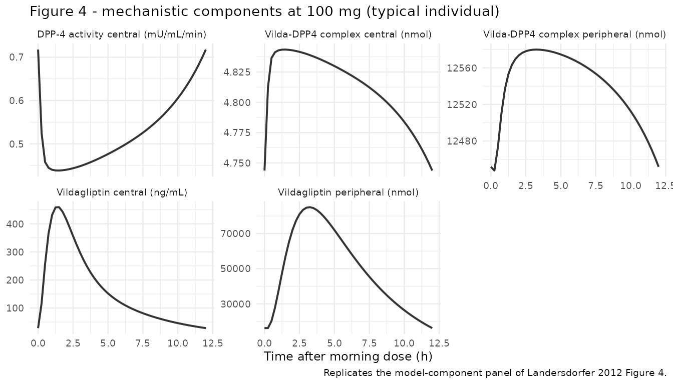
PKNCA validation
The paper reports terminal half-life (1.32 h at 10 mg, 2.43 h at 100 mg) and clearance computed as dose / AUC (84.0 L/h at 10 mg, 53.5 L/h at 100 mg), with the NCA carried out per subject by He et al. (Results section “Non-compartmental analysis”, citing ref [4]). We replicate per-subject NCA on the final BID interval and compare median values to the paper.
# Per-subject concentration table aligned to time-after-morning-dose,
# restricted to the last BID interval (0-12 h after the day-7 morning dose).
sim_nca <- sim |>
  dplyr::filter(!is.na(Cc), time >= sample_window) |>
  dplyr::transmute(
    id,
    time      = time - sample_window,
    Cc,
    treatment = factor(treatment, levels = c("10 mg", "25 mg", "100 mg"))
  )

# Defensive time-zero anchor (Cc = 0 wins only if no time=0 row already exists)
sim_nca <- dplyr::bind_rows(
  sim_nca,
  sim_nca |> dplyr::distinct(id, treatment) |>
    dplyr::mutate(time = 0, Cc = 0)
) |>
  dplyr::distinct(id, treatment, time, .keep_all = TRUE) |>
  dplyr::arrange(id, treatment, time)

# One representative dose per subject at the start of the interval; PKNCA
# uses it to compute dose-based parameters (CL, Vss, etc.).
dose_df <- sim_nca |>
  dplyr::distinct(id, treatment) |>
  dplyr::mutate(
    time = 0,
    amt = dplyr::case_when(
      treatment ==  "10 mg" ~  10,
      treatment ==  "25 mg" ~  25,
      treatment == "100 mg" ~ 100
    )
  )

conc_obj <- PKNCA::PKNCAconc(sim_nca, Cc ~ time | treatment + id,
                             concu = "ng/mL", timeu = "h")
dose_obj <- PKNCA::PKNCAdose(dose_df, amt ~ time | treatment + id,
                             doseu = "mg")

intervals <- data.frame(
  start     = 0,
  end       = 12,
  cmax      = TRUE,
  tmax      = TRUE,
  auclast   = TRUE,
  half.life = TRUE,
  cl.last   = TRUE
)

nca_res <- PKNCA::pk.nca(PKNCA::PKNCAdata(conc_obj, dose_obj, intervals = intervals))
Comparison against published NCA
The paper reports averaged NCA at the 10 mg and 100 mg doses (the 25 mg interval is not given a numeric value in the text). We compare per-subject medians from the simulation to the paper’s reported means. Cmax and AUC are not reported in the source for these dose levels (the paper directs the reader to He et al. ref [4]); only t1/2 and Dose/AUC clearance are quoted.
published <- tibble::tribble(
  ~treatment, ~half.life,
  "10 mg",    1.32,
  "100 mg",   2.43
)

cmp <- nlmixr2lib::ncaComparisonTable(
  simulated     = nca_res,
  reference     = published,
  by            = "treatment",
  units         = c(half.life = "h"),
  tolerance_pct = 20
)

knitr::kable(
  cmp,
  caption = "Simulated vs. published terminal half-life. * differs from reference by >20%.",
  align   = c("l", "l", "r", "r", "r")
)| NCA parameter | treatment | Reference | Simulated | % diff |
|---|---|---|---|---|
| t½ (h) | 10 mg | 1.32 | 2.44 | +85.1%* |
| t½ (h) | 100 mg | 2.43 | 2.45 | +1.0% |
Inspect the broader NCA output to confirm AUClast is consistent with the paper’s CL/F = Dose / AUC0-tau report (84.0 -> 53.5 L/h as the dose increases): increased AUC0-tau / dose at higher doses corresponds to lower apparent CL/F, the hallmark of saturable elimination by DPP-4.
nca_summary <- as.data.frame(nca_res$result) |>
  dplyr::filter(PPTESTCD %in% c("cmax", "tmax", "auclast", "half.life", "cl.last")) |>
  dplyr::group_by(treatment, PPTESTCD) |>
  dplyr::summarise(median = stats::median(PPORRES, na.rm = TRUE),
                   .groups = "drop") |>
  tidyr::pivot_wider(names_from = PPTESTCD, values_from = median)

knitr::kable(nca_summary,
             digits = c(0, 1, 2, 1, 2, 2),
             caption = "Median per-subject NCA over the day-7 BID interval (0-12 h post morning dose).",
align = "lrrrrr")| treatment | auclast | cl.last | cmax | half.life | tmax |
|---|---|---|---|---|---|
| 10 mg | 135.7 | 0.07 | 36.3 | 2.44 | 1.25 |
| 25 mg | 364.3 | 0.07 | 98.8 | 2.02 | 1.50 |
| 100 mg | 1816.1 | 0.06 | 429.6 | 2.45 | 1.50 |
Assumptions and deviations
- The original paper estimated a full variance-covariance matrix for the PK parameters in S-ADAPT, but Table 1 reports only the diagonal as BSV (%) = sqrt(omega^2) * 100. Off-diagonal covariances are not published, so the packaged model uses diagonal-only IIV. Joint draws are independent across parameters rather than correlated as in the original fit.
- Steady state for the day-28 sampling window is approximated by day 7 (= 13 BID doses). The slowest binding rate constant in the model is k_deg = 0.110 /h (t1/2 ~= 6.3 h), so by day 7 the system has cycled through ~ 27 half-lives and is at steady state to numerical precision; the system behaviour at day 7 is indistinguishable from day 28.
- The paper applied the Beal M3 method to handle vildagliptin concentrations below the LOQ (2 ng/mL) in S-ADAPT. The packaged model returns continuous concentrations without LOQ truncation; if you want to replicate the paper’s NCA at the 10 mg dose more faithfully, censor simulated Cc below 2 ng/mL before computing NCA (terminal half-life is sensitive to which late points are kept).
- Bioavailability F is fixed at 0.772 from co-modelling with the He YL
2007 intravenous-dose study; we keep that anchor
(
fixed(log(0.772))). - Initial conditions for all compartments are zero. At baseline (no vildagliptin) the DPP-4 activity equals cf1 * R_maxC = 2.80 * 5.0 = 14.0 mU/mL/min, consistent with the placebo DPP-4 activity envelope in Figure 3 of the source.
- The molecular weight used for the mg -> nmol dose conversion is 303.40 g/mol from PubChem (CID 6918537, C17H25N3O2). The paper itself does not state the MW; this value is the standard literature MW.
- Sequential absorption is encoded as
depot -> transit1 -> central. The paper’s two-rate-constant cascade with k_a1 != k_a2 (rather than a single Savic transit chain with shared ktr) is preserved by using two distinct log-transformed rate constants (lka1,lka2). - The peripheral drug-target complex compartment
(
complex_peripheral) is declared as apaper_specific_compartmentsentry because the canonical TMDDcomplex(Mager & Jusko 2001) covers single-site (central) binding only; Landersdorfer 2012 explicitly carries plasma + tissue binding as two separate complex states.