Rivipansel (Tammara 2017)
Source:vignettes/articles/Tammara_2017_rivipansel.Rmd
Tammara_2017_rivipansel.RmdModel and source
The integrated population PK model published by Tammara and Harnisch (2017) was used to inform the rivipansel phase III dose-selection exercise in pediatric patients with sickle cell disease (SCD). The model pools 109 subjects from three rivipansel phase I studies and the phase II study (NCT01119833) in adolescents and adults hospitalized for vaso-occlusive crisis (VOC). It is a three-compartment IV linear disposition model with creatinine clearance and body weight as the only structural covariates.
- Citation: Tammara BK, Harnisch LO. Dose Selection Based on Modeling and Simulation for Rivipansel in Pediatric Patients Aged 6 to 11 Years With Sickle Cell Disease. CPT Pharmacometrics Syst Pharmacol. 2017;6(12):845-854.
- Article: https://doi.org/10.1002/psp4.12263
Population
The integrated dataset pooled 109 subjects aged 12-51 years across four studies: rivipansel study 101 (single IV dose 2-40 mg/kg in healthy adults, n = 40), study 102 (multiple IV doses 2-20 mg/kg q8h plus a 40 mg/kg loading dose followed by 20 mg/kg q8h in healthy adults, n = 32), study 103 / NCT00911495 (two IV doses 20 mg/kg loading + 10 mg/kg in adults with SCD not in VOC, n = 15), and the phase II study NCT01119833 (Telen 2015) in patients with SCD aged 12-60 years hospitalized for VOC, n = 76 (56 adults and 20 children aged 12-17 years). Rivipansel is renally cleared with about 60% protein binding and a low volume of distribution; phase I half-life is approximately 7-8 hours.
The same population metadata is available programmatically:
readModelDb("Tammara_2017_rivipansel")$populationSource trace
Every ini() value carries a trailing comment in
inst/modeldb/specificDrugs/Tammara_2017_rivipansel.R
pointing to its source location. The table below collects them for
review.
| Equation / parameter | Value | Source location |
|---|---|---|
| Three-compartment IV linear disposition with central + peripheral1 + peripheral2 | – | Methods, “Study design and data sources” |
| Typical CL = 1.25 * (CRCL/150)^0.468 * (1 + 0.234 * STUD) | – | Table 1 footnote b |
| Typical V1 = 6.24 * (WT/70)^0.569 | – | Table 1 footnote c |
| Typical V2 = 4.02 * (WT/70)^0.569 | – | Table 1 footnote c |
| Typical V3 = 0.656 * (WT/70)^0.569 | – | Table 1 footnote c |
lcl (CL, L/h) |
1.25 | Table 1, CL row |
lvc (V1, L) |
6.24 | Table 1, V1 row |
lq (Q_rapid, L/h) |
2.62 | Table 1, Q_rapid row |
lvp (V2, L) |
4.02 | Table 1, V2 row |
lq2 (Q_slow, L/h) |
0.0316 | Table 1, Q_slow row |
lvp2 (V3, L) |
0.656 | Table 1, V3 row |
e_study_riv201_cl (additive SCD shift, fraction) |
0.234 | Table 1, “Study effect on CL” row |
e_crcl_cl (CRCL exponent on CL) |
0.468 | Table 1, “Exponent for CRCL on CL” row |
e_wt_vc_vp_vp2 (shared WT exponent) |
0.569 | Table 1, “Exponent for WT on V1, V2, V3” row |
| IIV %CV on CL / V1 / Q_rapid / V2 / Q_slow / V3 | 18.8 / 24.1 / 19.8 / 15.5 / 15.5 / 15.3 | Table 1, interindividual variability rows |
| Additive residual SD (phase I / study 201) | 0.29 / 0.165 ug/mL | Table 1, residual variability rows |
| Proportional residual %CV (phase I / study 201) | 9.52 / 23.2 | Table 1, residual variability rows |
Virtual cohort
The original observed data are not publicly available. The cohort
below approximates the phase II SCD population, with body weight and
creatinine clearance distributions drawn from typical SCD-cohort ranges
and STUDY_RIV201 set to 1 for every subject (the simulation
target is the SCD population for which the dose-selection exercise
applies).
set.seed(12263)  # DOI suffix
n_subj <- 100

# Body weight (kg). Phase II included adolescents and adults; weight
# distribution sampled to span a typical adolescent-adult SCD range
# (Tammara 2017 Figure 2; observed phase II weights ranged roughly
# 40-110 kg with median near 70 kg).
WT <- pmin(pmax(rnorm(n_subj, mean = 70, sd = 15), 45), 110)

# Creatinine clearance (mL/min, NOT BSA-normalized; raw Cockcroft-Gault
# scale per Tammara 2017). SCD hyperfiltration shifts the typical CRCL
# in adults upward of the 120 mL/min anchor; the simulated distribution
# centres on 130 mL/min and spans 60-200 mL/min, matching the observed
# range in Tammara 2017 Figure 4 (adult panel).
CRCL <- pmin(pmax(rnorm(n_subj, mean = 130, sd = 30), 60), 200)

# Phase II SCD study indicator: 1 for every subject in the target
# population (the simulation context is the SCD cohort).
STUDY_RIV201 <- rep(1L, n_subj)

cohort <- tibble(
  id           = seq_len(n_subj),
  WT           = WT,
  CRCL         = CRCL,
  STUDY_RIV201 = STUDY_RIV201
)
Simulation
Rivipansel is administered as a 20-minute IV infusion. The dose-selection regimen recommended by Tammara 2017 for phase III is a 40 mg/kg loading dose followed by 20 mg/kg every 12 hours; we simulate that regimen out to seven days so steady state is reached.
infusion_dur <- 20 / 60  # 20 minutes expressed in hours
tau          <- 12       # dosing interval (hours)
maint_doses  <- 13       # 13 maintenance doses after loading -> 14 doses, 7 days

# Per-subject dosing: loading dose at time 0, then maintenance doses
# at 12-hour intervals. amt is in mg (weight-based mg/kg dose times
# subject weight); rate is amt / 20-min infusion duration.
make_doses <- function(row) {
  load_amt  <- 40 * row$WT
  maint_amt <- 20 * row$WT
  dose_times <- c(0, tau * seq_len(maint_doses))
  amt        <- c(load_amt, rep(maint_amt, maint_doses))
  data.frame(
    id           = row$id,
    time         = dose_times,
    amt          = amt,
    rate         = amt / infusion_dur,
    evid         = 1L,
    cmt          = "central",
    WT           = row$WT,
    CRCL         = row$CRCL,
    STUDY_RIV201 = row$STUDY_RIV201
  )
}

doses <- cohort |>
  split(seq_len(nrow(cohort))) |>
  lapply(make_doses) |>
  bind_rows()

# Observation grid: every 0.5 h for the first 24 h to characterise the
# loading-dose phase, then every 2 h out to 168 h (7 days). The final
# dosing interval (156-168 h) is the steady-state window used for NCA.
obs_times <- sort(unique(c(
  seq(0, 24, by = 0.5),
  seq(24, 168, by = 2)
)))
obs <- expand_grid(
  id = cohort$id,
  time = obs_times
) |>
  mutate(amt = NA_real_, rate = NA_real_, evid = 0L, cmt = "central") |>
  left_join(cohort, by = "id")

events <- bind_rows(doses, obs) |>
  arrange(id, time, desc(evid))
stopifnot(!anyDuplicated(unique(events[, c("id", "time", "evid")])))
mod <- readModelDb("Tammara_2017_rivipansel")
sim <- rxode2::rxSolve(mod, events = events,
                       keep = c("WT", "CRCL", "STUDY_RIV201")) |>
  as.data.frame() |>
  filter(!is.na(Cc))
#> ℹ parameter labels from comments will be replaced by 'label()'
Replicate published figures
# Approximate Tammara 2017 Figure 5 (adult panel column on the 40/20
# mg/kg regimen): predicted concentration-time trajectory in adult SCD
# subjects on the recommended regimen. Median and 5th/95th prediction
# intervals over 168 h.
sim |>
  group_by(time) |>
  summarise(
    Q05 = quantile(Cc, 0.05, na.rm = TRUE),
    Q50 = quantile(Cc, 0.50, na.rm = TRUE),
    Q95 = quantile(Cc, 0.95, na.rm = TRUE),
    .groups = "drop"
  ) |>
  ggplot(aes(time, Q50)) +
  geom_ribbon(aes(ymin = Q05, ymax = Q95), alpha = 0.25, fill = "steelblue") +
  geom_line(colour = "steelblue4") +
  geom_hline(yintercept = 10, linetype = "dashed", colour = "red") +
  scale_y_log10() +
  labs(
    x = "Time (h)",
    y = "Rivipansel concentration (ug/mL)",
    title = "Adult SCD prediction interval on 40/20 mg/kg q12h",
    caption = paste(
      "Replicates the adult panel of Tammara 2017 Figure 5 (rightmost",
      "row; 40/20 mg/kg regimen). Dashed line: 10 ug/mL preclinical",
      "efficacy threshold."
    )
  )
#> Warning in scale_y_log10(): log-10 transformation introduced infinite values.
#> log-10 transformation introduced infinite values.
#> log-10 transformation introduced infinite values.
#> log-10 transformation introduced infinite values.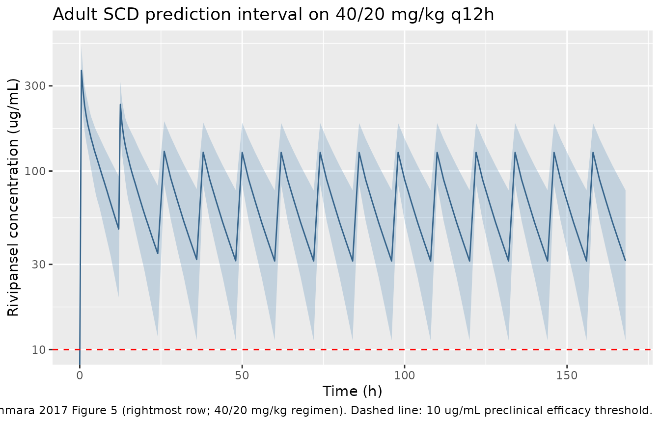
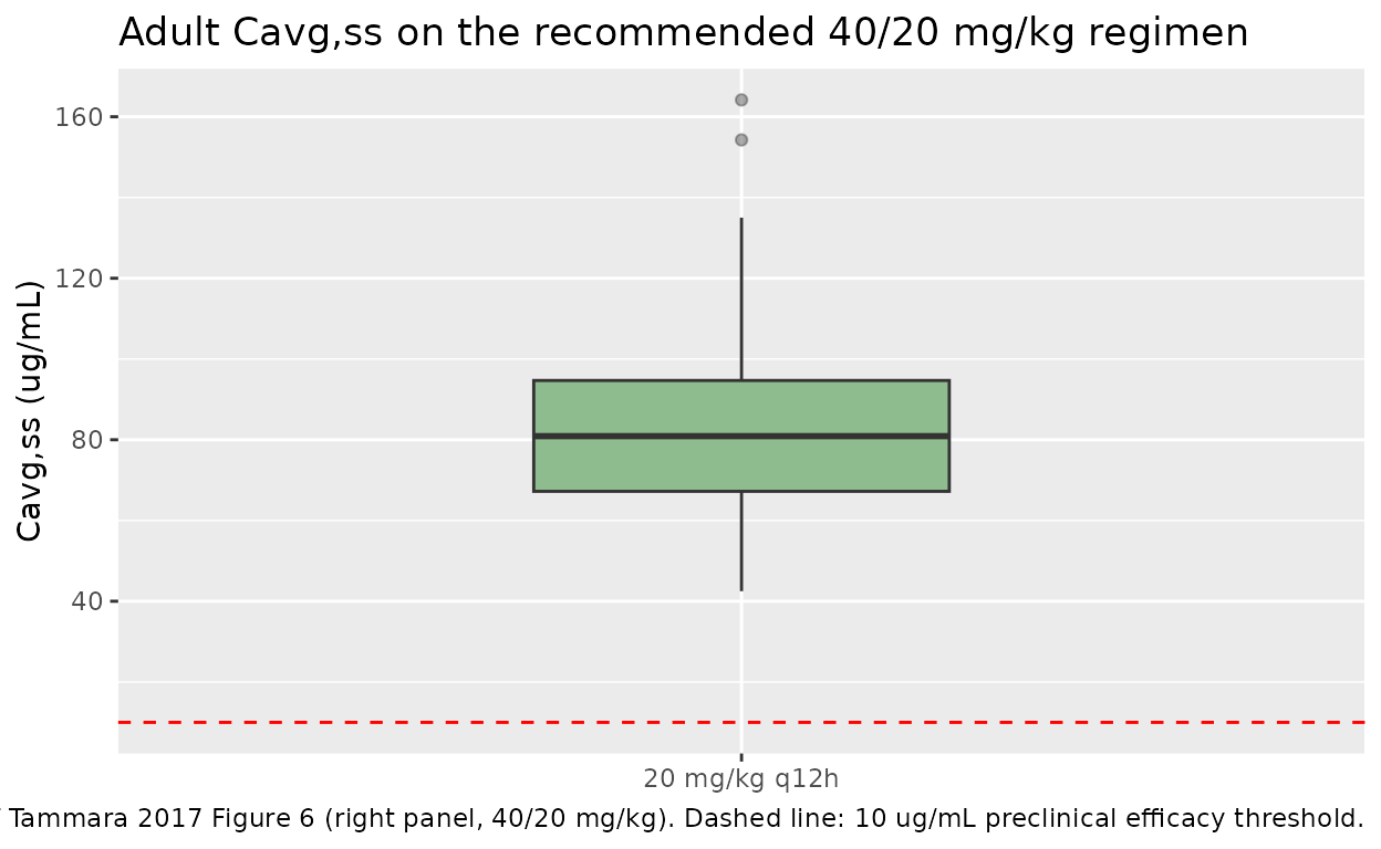
# Approximate Tammara 2017 Figure 6 (high-dose panel for adults): the
# Cavg,ss distribution in adults on the 20 mg/kg q12h maintenance
# regimen. Computed analytically from each subject's individual CL
# rather than from the simulated concentration trace (per the paper:
# "Cavg,ss simulations did not contain residual error as they reflect
# a model-based summary measure across the whole dosing interval").
mod_typical <- mod  # individual CL from simulation already includes IIV
cavg_ss <- sim |>
  group_by(id) |>
  slice(1) |>
  ungroup() |>
  mutate(
    maint_amt = 20 * WT,
    cl_i      = exp(log(1.25)) * (CRCL / 150)^0.468 *
                  (1 + 0.234 * STUDY_RIV201),
    Cavg_ss   = (maint_amt / tau) / cl_i
  )

ggplot(cavg_ss, aes(x = "20 mg/kg q12h", y = Cavg_ss)) +
  geom_boxplot(fill = "darkseagreen", width = 0.4, outlier.alpha = 0.4) +
  geom_hline(yintercept = 10, linetype = "dashed", colour = "red") +
  labs(
    x = NULL,
    y = "Cavg,ss (ug/mL)",
    title = "Adult Cavg,ss on the recommended 40/20 mg/kg regimen",
    caption = paste(
      "Replicates the adult-panel portion of Tammara 2017 Figure 6",
      "(right panel, 40/20 mg/kg). Dashed line: 10 ug/mL preclinical",
      "efficacy threshold."
    )
  )
PKNCA validation
Validation against the published Cavg,ss summary (Figure 6) and the phase I terminal half-life (Methods narrative: mean phase I half-life 7-8 hours). The steady-state NCA window is the final dosing interval (156-168 h) at the 20 mg/kg q12h maintenance dose; results are grouped by the single treatment label.
sim_nca <- sim |>
  mutate(treatment = "40/20 mg/kg q12h") |>
  select(id, time, Cc, treatment)

dose_df <- events |>
  filter(evid == 1) |>
  mutate(treatment = "40/20 mg/kg q12h") |>
  select(id, time, amt, treatment)

conc_obj <- PKNCA::PKNCAconc(
  sim_nca, Cc ~ time | treatment + id,
  concu = "ug/mL", timeu = "hour"
)
dose_obj <- PKNCA::PKNCAdose(
  dose_df, amt ~ time | treatment + id,
  doseu = "mg"
)

start_ss <- max(dose_df$time)
end_ss   <- start_ss + tau

intervals <- data.frame(
  start    = c(0,        start_ss),
  end      = c(tau,      end_ss),
  cmax     = c(TRUE,     TRUE),
  tmax     = c(TRUE,     TRUE),
  cmin     = c(FALSE,    TRUE),
  auclast  = c(TRUE,     TRUE),
  cav      = c(FALSE,    TRUE),
  ctrough  = c(FALSE,    TRUE)
)

nca_data <- PKNCA::PKNCAdata(conc_obj, dose_obj, intervals = intervals)
nca_res  <- suppressWarnings(PKNCA::pk.nca(nca_data))

nca_tbl <- as.data.frame(nca_res$result)
nca_summary <- nca_tbl |>
  group_by(PPTESTCD, start, end) |>
  summarise(
    median = median(PPORRES, na.rm = TRUE),
    q05    = quantile(PPORRES, 0.05, na.rm = TRUE),
    q95    = quantile(PPORRES, 0.95, na.rm = TRUE),
    .groups = "drop"
  ) |>
  arrange(start, PPTESTCD)

knitr::kable(
  nca_summary,
  digits = 3,
  caption = paste(
    "Simulated NCA parameters for the 40/20 mg/kg q12h regimen.",
    "Start = 0 covers the loading-dose interval; start =", start_ss,
    "covers the steady-state interval (last maintenance dose +",
    tau, "h)."
  )
)| PPTESTCD | start | end | median | q05 | q95 |
|---|---|---|---|---|---|
| auclast | 0 | 12 | 1505.556 | 906.185 | 2119.149 |
| cmax | 0 | 12 | 366.095 | 264.191 | 558.341 |
| tmax | 0 | 12 | 0.500 | 0.500 | 0.500 |
| auclast | 156 | 168 | 822.115 | 382.787 | 1382.404 |
| cav | 156 | 168 | 68.510 | 31.899 | 115.200 |
| cmax | 156 | 168 | 126.654 | 74.696 | 186.273 |
| cmin | 156 | 168 | 30.461 | 9.720 | 72.098 |
| ctrough | 156 | 168 | NA | NA | NA |
| tmax | 156 | 168 | 2.000 | 2.000 | 2.000 |
Terminal half-life from a single-dose simulation
The paper reports a mean phase I terminal half-life of 7-8 hours. To
verify the model reproduces that value, simulate a single 40 mg/kg dose
in a typical 70-kg phase I subject (STUDY_RIV201 = 0,
CRCL = 100) and compute the terminal half-life via
PKNCA.
typ <- tibble(
  id           = 1L,
  WT           = 70,
  CRCL         = 100,
  STUDY_RIV201 = 0L
)

typ_events <- bind_rows(
  data.frame(
    id   = 1L, time = 0, amt = 40 * 70,
    rate = (40 * 70) / infusion_dur, evid = 1L, cmt = "central",
    WT = 70, CRCL = 100, STUDY_RIV201 = 0L
  ),
  data.frame(
    id   = 1L, time = seq(0, 72, by = 0.25),
    amt = NA_real_, rate = NA_real_, evid = 0L, cmt = "central",
    WT = 70, CRCL = 100, STUDY_RIV201 = 0L
  )
) |>
  arrange(time, desc(evid))

mod_zero <- rxode2::zeroRe(mod)
#> ℹ parameter labels from comments will be replaced by 'label()'
#> Warning: No sigma parameters in the model
typ_sim <- rxode2::rxSolve(mod_zero, events = typ_events,
                           keep = c("WT", "CRCL", "STUDY_RIV201")) |>
  as.data.frame() |>
  filter(!is.na(Cc)) |>
  mutate(id = 1L, treatment = "single 40 mg/kg")
#> ℹ omega/sigma items treated as zero: 'etalcl', 'etalvc', 'etalq', 'etalvp', 'etalq2', 'etalvp2'

conc_obj_typ <- PKNCA::PKNCAconc(
  typ_sim |> select(id, time, Cc, treatment),
  Cc ~ time | treatment + id,
  concu = "ug/mL", timeu = "hour"
)
dose_obj_typ <- PKNCA::PKNCAdose(
  data.frame(id = 1L, time = 0, amt = 40 * 70,
             treatment = "single 40 mg/kg"),
  amt ~ time | treatment + id,
  doseu = "mg"
)
intervals_typ <- data.frame(
  start      = 0,
  end        = Inf,
  cmax       = TRUE,
  tmax       = TRUE,
  aucinf.obs = TRUE,
  half.life  = TRUE
)
nca_typ <- suppressWarnings(PKNCA::pk.nca(
  PKNCA::PKNCAdata(conc_obj_typ, dose_obj_typ, intervals = intervals_typ)
))
typ_tbl <- as.data.frame(nca_typ$result) |>
  select(PPTESTCD, PPORRES)
knitr::kable(
  typ_tbl,
  digits = 3,
  caption = "Typical-value NCA after a single 40 mg/kg IV infusion in a phase I 70-kg subject (CRCL = 100 mL/min)."
)| PPTESTCD | PPORRES |
|---|---|
| cmax | 375.000 |
| tmax | 0.500 |
| tlast | 72.000 |
| clast.obs | 0.626 |
| lambda.z | 0.063 |
| r.squared | 1.000 |
| adj.r.squared | 1.000 |
| lambda.z.time.first | 64.750 |
| lambda.z.time.last | 72.000 |
| lambda.z.n.points | 30.000 |
| clast.pred | 0.625 |
| half.life | 11.012 |
| span.ratio | 0.658 |
| aucinf.obs | 2696.668 |
The published phase I mean half-life of 7-8 hours is the comparator
against the half.life row above.
Assumptions and deviations
- The phase II SCD residual error magnitudes
(
addSd_study201,propSd_study201) and the phase I magnitudes (addSd_phase1,propSd_phase1) are estimated separately in Tammara 2017 Table 1. The model file selects between them per observation via theSTUDY_RIV201indicator. Simulations targeting the SCD population useSTUDY_RIV201 = 1, which selectspropSd = 0.232,addSd = 0.165 ug/mL. - Tammara 2017 expresses CRCL in raw mL/min (Cockcroft-Gault for
adults, Schwartz with BSA adjustment for children to give an absolute
mL/min value), not normalised to 1.73 m^2. The canonical
CRCLcovariate accepts both conventions; this model file’scovariateData[[CRCL]]$unitsis"mL/min"to flag the non-BSA-normalised use. - Body weight and CRCL distributions for the virtual cohort are approximated from the figures in the paper (Figure 2 for weight, Figure 4 for creatinine clearance in adults). The exact baseline demographics table for the integrated dataset is not reproduced in the publication.
- The Cavg,ss distribution figure uses the closed-form Cavg,ss = (dose / tau) / CL_i per subject, matching the paper’s approach (“Cavg,ss simulations did not contain residual error as they reflect a model-based summary measure across the whole dosing interval”).
- The model does not encode the pediatric (6-11 year) demographic extrapolation from the CDC growth charts and the Hoste creatinine relationship that the paper develops for its simulation exercise. Users extrapolating to younger pediatric populations must supply the appropriate WT, CRCL covariate values themselves; the structural model and the SCD hyperfiltration effect are assumed by the paper to apply unchanged in younger children.
- No
etacorrelation structure was reported in Table 1; the six IIV terms are encoded as independent log-normal random effects.