Clindamycin (Mimram 2022)
Source:vignettes/articles/Mimram_2022_clindamycin.Rmd
Mimram_2022_clindamycin.RmdModel and source
- Citation: Mimram L, Magreault S, Kerroumi Y, Salmon D, Kably B, Marmor S, Jannot A-S, Jullien V, Zeller V. Population Pharmacokinetics of Orally Administered Clindamycin to Treat Prosthetic Joint Infections: A Prospective Study. Antibiotics (Basel). 2022;11(11):1462. doi:10.3390/antibiotics11111462
- Description: One-compartment population PK model with first-order absorption and elimination for orally administered clindamycin in adults with chronic prosthetic joint infections not receiving rifampicin; no covariates retained (Mimram 2022).
- Article: https://doi.org/10.3390/antibiotics11111462 (open access)
Population
Mimram et al. analysed 140 plasma clindamycin concentrations from 20 adults treated for a chronic prosthetic joint infection (14 hip, 3 knee and 3 shoulder arthroplasties) in Paris, France, between December 2015 and November 2019 (NCT02629770). Only patients not prescribed rifampicin were included. The cohort was 13 men and 7 women, with mean (SD) age 66.5 (15.9) years and body weight 76.3 (14.4) kg (Table 1). Patients with hepatocellular insufficiency, cirrhosis, creatinine clearance below 30 mL/min, body weight outside 50-100 kg, severe sepsis, or CYP3A4/5-interacting co-medication were excluded.
After 2-5 weeks of intravenous clindamycin, patients took oral clindamycin 750 mg q8h (< 80 kg) or 900 mg q8h (>= 80 kg; up to 1200 mg q8h above 95 kg). After 2 weeks of oral dosing, seven samples were drawn across one dosing interval (0, 0.5, 1, 2, 4, 6 and 8 h). Observed concentrations ranged from 0.4 to 13.5 mg/L.
The same information is available programmatically via
readModelDb("Mimram_2022_clindamycin")()$population.
Source trace
| Equation / parameter | Value | Source location |
|---|---|---|
| Structure: one compartment, first-order absorption and elimination | n/a | Section 2.2; Abstract |
lka |
log(3.53) 1/h |
Table 2, Ka |
lcl |
log(23) L/h |
Table 2, CL/F |
lvc |
log(103) L |
Table 2, V/F |
etalcl |
variance 0.144 | Table 2 omega2 CL/F = 0.14; Abstract 14.4% |
etalvc |
variance 0.082 | Table 2 omega2 V/F = 0.08; Abstract 8.2% |
etalka |
variance 0.596 | Table 2 omega2 Ka = 0.60; Abstract 59.6% |
propSd |
0.0988 (= sqrt(0.00976)) | Table 2, proportional error |
addSd |
0.283 mg/L (= sqrt(0.0801)) | Table 2, additive error |
| Covariates | none retained | Section 2.2 (sex, age, weight, height, bilirubin, creatinine and ALT screened; Section 4.7) |
d/dt(depot), d/dt(central),
Cc = central / vc
|
n/a | Standard one-compartment oral model, Section 2.2 |
Steady-state regimens of Table 3
Table 3 of the paper reports Monte Carlo steady-state trough concentrations (median and 90% interval) and target-attainment probabilities for seven oral regimens. Each regimen below gets its own cohort of 200 virtual patients. The model has no covariates, so no demographic distribution is needed. Doses are given until 96 h, which is more than ten typical half-lives, and the interval after the 96 h dose is observed densely.
rxode2::rxSetSeed(20221023)

regimens <- tibble::tribble(
  ~regimen,       ~dose, ~tau,
  "450 mg q6h",     450,    6,
  "600 mg q8h",     600,    8,
  "600 mg q6h",     600,    6,
  "750 mg q8h",     750,    8,
  "750 mg q6h",     750,    6,
  "900 mg q8h",     900,    8,
  "900 mg q6h",     900,    6
)
n_per_arm <- 200L
t_last_dose <- 96

make_regimen <- function(regimen, dose, tau, id_offset) {
  ids <- id_offset + seq_len(n_per_arm)
  dose_times <- seq(0, t_last_dose, by = tau)
  obs_times <- t_last_dose + c(0, 0.25, 0.5, 1, 1.5, 2, 3, 4, 5, 6, 7, 8)
  obs_times <- obs_times[obs_times <= t_last_dose + tau]
  doses <- tidyr::expand_grid(id = ids, time = dose_times) |>
    dplyr::mutate(evid = 1L, amt = dose, cmt = "depot")
  obs <- tidyr::expand_grid(id = ids, time = obs_times) |>
    dplyr::mutate(evid = 0L, amt = 0, cmt = "central")
  dplyr::bind_rows(doses, obs) |>
    dplyr::mutate(regimen = regimen, tau = tau, dose = dose) |>
    dplyr::arrange(id, time, dplyr::desc(evid))
}

events <- dplyr::bind_rows(lapply(seq_len(nrow(regimens)), function(i) {
  make_regimen(
    regimens$regimen[i], regimens$dose[i], regimens$tau[i],
    id_offset = (i - 1L) * n_per_arm
  )
}))
stopifnot(!anyDuplicated(unique(events[, c("id", "time", "evid")])))
mod <- readModelDb("Mimram_2022_clindamycin")
sim <- rxode2::rxSolve(mod, events = events, keep = c("regimen", "tau")) |>
  as.data.frame()
#> ℹ parameter labels from comments will be replaced by 'label()'
Typical-value check against the closed form
With the random effects removed, the steady-state trough of a one-compartment oral model has a closed form. The ODE solve should agree with it to numerical precision. This check uses the same parameters on both sides, so a tight bound is appropriate.
sim_typ <- rxode2::rxSolve(rxode2::zeroRe(mod), events = events, keep = c("regimen", "tau")) |>
  as.data.frame()
#> ℹ parameter labels from comments will be replaced by 'label()'
#> ℹ omega/sigma items treated as zero: 'etalcl', 'etalvc', 'etalka'
#> Warning: multi-subject simulation without without 'omega'

ss_trough <- function(dose, tau, cl = 23, v = 103, ka = 3.53) {
  k <- cl / v
  dose / v * ka / (ka - k) *
    (exp(-k * tau) / (1 - exp(-k * tau)) - exp(-ka * tau) / (1 - exp(-ka * tau)))
}

typ_check <- sim_typ |>
  dplyr::filter(time == t_last_dose + tau) |>
  dplyr::distinct(regimen, tau, Cc) |>
  dplyr::left_join(regimens, by = c("regimen", "tau")) |>
  dplyr::mutate(closed_form = ss_trough(dose, tau), rel_err = Cc / closed_form - 1)
knitr::kable(typ_check |> dplyr::select(regimen, Cc, closed_form, rel_err), digits = 4)| regimen | Cc | closed_form | rel_err |
|---|---|---|---|
| 450 mg q6h | 1.6549 | 1.6549 | 0 |
| 600 mg q8h | 1.2517 | 1.2517 | 0 |
| 600 mg q6h | 2.2065 | 2.2065 | 0 |
| 750 mg q8h | 1.5647 | 1.5647 | 0 |
| 750 mg q6h | 2.7581 | 2.7581 | 0 |
| 900 mg q8h | 1.8776 | 1.8776 | 0 |
| 900 mg q6h | 3.3098 | 3.3098 | 0 |
Concentration-time profiles at steady state
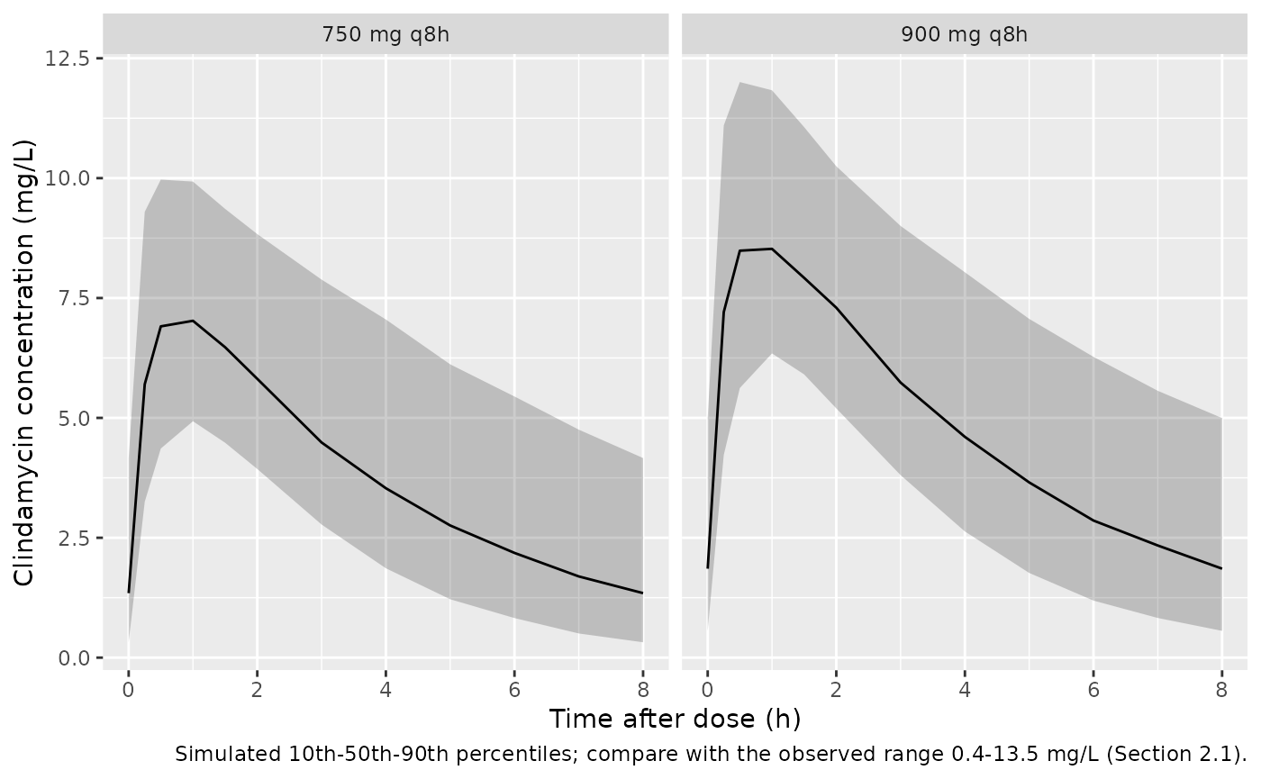
Figure 2 of the paper is a prediction- and variability-corrected VPC of the observed data, which are not public. The plot below shows the simulated 10th, 50th and 90th percentiles (the percentiles Figure 2 uses) over one steady-state interval for the two regimens given in the study.
sim |>
  dplyr::filter(regimen %in% c("750 mg q8h", "900 mg q8h")) |>
  dplyr::mutate(tad = time - t_last_dose) |>
  dplyr::group_by(regimen, tad) |>
  dplyr::summarise(
    Q10 = quantile(Cc, 0.10),
    Q50 = quantile(Cc, 0.50),
    Q90 = quantile(Cc, 0.90),
    .groups = "drop"
  ) |>
  ggplot(aes(tad, Q50)) +
  geom_ribbon(aes(ymin = Q10, ymax = Q90), alpha = 0.25) +
  geom_line() +
  facet_wrap(~regimen) +
  labs(
    x = "Time after dose (h)", y = "Clindamycin concentration (mg/L)",
    caption = "Simulated 10th-50th-90th percentiles; compare with the observed range 0.4-13.5 mg/L (Section 2.1)."
  )
PKNCA validation
PKNCA computes the steady-state Cmax, Cmin and AUC0-tau over the
interval after the 96 h dose. At steady state, cmin is the
trough concentration that Table 3 reports.
sim_nca <- sim |>
  dplyr::filter(!is.na(Cc)) |>
  dplyr::select(id, time, Cc, regimen)

dose_df <- events |>
  dplyr::filter(evid == 1) |>
  dplyr::select(id, time, amt, regimen)

conc_obj <- PKNCA::PKNCAconc(sim_nca, Cc ~ time | regimen + id)
dose_obj <- PKNCA::PKNCAdose(dose_df, amt ~ time | regimen + id)

intervals <- regimens |>
  dplyr::transmute(
    regimen,
    start = t_last_dose,
    end = t_last_dose + tau,
    cmax = TRUE,
    tmax = TRUE,
    cmin = TRUE,
    auclast = TRUE
  ) |>
  as.data.frame()

nca_res <- PKNCA::pk.nca(PKNCA::PKNCAdata(conc_obj, dose_obj, intervals = intervals))
Comparison against Table 3 trough concentrations
published <- tibble::tribble(
  ~regimen,       ~cmin,
  "450 mg q6h",    1.73,
  "600 mg q8h",    1.31,
  "600 mg q6h",    2.10,
  "750 mg q8h",    1.51,
  "750 mg q6h",    2.81,
  "900 mg q8h",    1.92,
  "900 mg q6h",    3.38
)

cmp <- nlmixr2lib::ncaComparisonTable(
  simulated = nca_res,
  reference = published,
  by = "regimen",
  params = "cmin",
  units = c(cmin = "mg/L"),
  tolerance_pct = 20
)
knitr::kable(cmp, caption = "Simulated vs. published median steady-state trough (Table 3). * differs by >20%.")| NCA parameter | regimen | Reference | Simulated | % diff |
|---|---|---|---|---|
| Cmin (mg/L) | 450 mg q6h | 1.73 | 1.84 | +6.5% |
| Cmin (mg/L) | 600 mg q8h | 1.31 | 1.22 | -7.2% |
| Cmin (mg/L) | 600 mg q6h | 2.1 | 2.12 | +1.2% |
| Cmin (mg/L) | 750 mg q8h | 1.51 | 1.35 | -10.9% |
| Cmin (mg/L) | 750 mg q6h | 2.81 | 2.84 | +1.0% |
| Cmin (mg/L) | 900 mg q8h | 1.92 | 1.86 | -3.4% |
| Cmin (mg/L) | 900 mg q6h | 3.38 | 3.12 | -7.7% |
The paper reports the 90% interval of the simulated troughs alongside
the median. The intervals below come from the same simulated
cmin values.
troughs <- as.data.frame(nca_res$result) |>
  dplyr::filter(PPTESTCD == "cmin") |>
  dplyr::select(id, regimen, trough = PPORRES)

published_ci <- tibble::tribble(
  ~regimen,      ~pub_median, ~pub_lo, ~pub_hi,
  "450 mg q6h",         1.73,    0.42,    4.10,
  "600 mg q8h",         1.31,    0.21,    4.67,
  "600 mg q6h",         2.10,    0.41,    5.51,
  "750 mg q8h",         1.51,    0.19,    4.92,
  "750 mg q6h",         2.81,    0.63,    6.73,
  "900 mg q8h",         1.92,    0.31,    5.89,
  "900 mg q6h",         3.38,    0.71,    8.55
)

trough_summary <- troughs |>
  dplyr::group_by(regimen) |>
  dplyr::summarise(
    sim_median = median(trough),
    sim_lo = quantile(trough, 0.05),
    sim_hi = quantile(trough, 0.95),
    .groups = "drop"
  ) |>
  dplyr::left_join(published_ci, by = "regimen") |>
  dplyr::mutate(pct_diff = 100 * (sim_median / pub_median - 1))

trough_summary |>
  dplyr::select(regimen, sim_median, pub_median, sim_lo, pub_lo, sim_hi, pub_hi) |>
  dplyr::rename(
    "Regimen" = regimen,
    "Median (sim)" = sim_median, "Median (Table 3)" = pub_median,
    "5th pct (sim)" = sim_lo, "5th pct (Table 3)" = pub_lo,
    "95th pct (sim)" = sim_hi, "95th pct (Table 3)" = pub_hi
  ) |>
knitr::kable(digits = 2, caption = "Steady-state trough (mg/L): median and 90% interval.")| Regimen | Median (sim) | Median (Table 3) | 5th pct (sim) | 5th pct (Table 3) | 95th pct (sim) | 95th pct (Table 3) |
|---|---|---|---|---|---|---|
| 450 mg q6h | 1.84 | 1.73 | 0.41 | 0.42 | 4.50 | 4.10 |
| 600 mg q6h | 2.12 | 2.10 | 0.49 | 0.41 | 5.85 | 5.51 |
| 600 mg q8h | 1.22 | 1.31 | 0.21 | 0.21 | 3.54 | 4.67 |
| 750 mg q6h | 2.84 | 2.81 | 0.58 | 0.63 | 7.29 | 6.73 |
| 750 mg q8h | 1.35 | 1.51 | 0.26 | 0.19 | 5.03 | 4.92 |
| 900 mg q6h | 3.12 | 3.38 | 0.73 | 0.71 | 8.38 | 8.55 |
| 900 mg q8h | 1.86 | 1.92 | 0.38 | 0.31 | 5.91 | 5.89 |
Probability of target attainment (Table 3)
The trough targets are 2 x MIC and 8 x MIC, plus an upper limit of 5 mg/L. The paper does not say whether residual error was added to the simulated troughs. Adding the combined residual error changes these probabilities by at most a few percentage points, so the comparison below uses the individual predictions.
mics <- c(0.5, 0.25, 0.125, 0.0625, 0.03125)

sim_pta <- tidyr::expand_grid(troughs, mic = mics) |>
  dplyr::group_by(regimen, mic) |>
  dplyr::summarise(
    `2x MIC` = 100 * mean(trough >= 2 * mic),
    `8x MIC` = 100 * mean(trough >= 8 * mic),
    .groups = "drop"
  ) |>
  tidyr::pivot_longer(c(`2x MIC`, `8x MIC`), names_to = "target", values_to = "sim")

pub_pta <- tibble::tribble(
  ~target,  ~mic,     ~`450 mg q6h`, ~`600 mg q8h`, ~`600 mg q6h`, ~`750 mg q8h`, ~`750 mg q6h`, ~`900 mg q8h`, ~`900 mg q6h`,
  "2x MIC", 0.5,      75, 64, 81, 70,  89, 76,  92,
  "2x MIC", 0.25,     93, 86, 94, 85,  97, 91,  98,
  "2x MIC", 0.125,    97, 93, 97, 93,  99, 97,  99,
  "2x MIC", 0.0625,   99, 97, 99, 97, 100, 99, 100,
  "2x MIC", 0.03125, 100, 99, 100, 98, 100, 99, 100,
  "8x MIC", 0.5,       6,  8, 16,  9,  29, 15,  38,
  "8x MIC", 0.25,     39, 30, 53, 37,  68, 48,  74,
  "8x MIC", 0.125,    75, 64, 81, 70,  89, 76,  92,
  "8x MIC", 0.0625,   93, 86, 94, 85,  97, 91,  98,
  "8x MIC", 0.03125,  97, 93, 97, 93,  99, 97,  99
) |>
  tidyr::pivot_longer(-c(target, mic), names_to = "regimen", values_to = "published")

pta_cmp <- dplyr::inner_join(sim_pta, pub_pta, by = c("regimen", "mic", "target")) |>
  dplyr::mutate(diff = sim - published)

pta_cmp |>
  dplyr::mutate(cell = sprintf("%.0f (%.0f)", sim, published)) |>
  dplyr::select(target, mic, regimen, cell) |>
  tidyr::pivot_wider(names_from = regimen, values_from = cell) |>
  dplyr::rename("Target" = target, "MIC (mg/L)" = mic) |>
knitr::kable(caption = "PTA (%): simulated (Table 3 in parentheses).")| Target | MIC (mg/L) | 450 mg q6h | 600 mg q6h | 600 mg q8h | 750 mg q6h | 750 mg q8h | 900 mg q6h | 900 mg q8h |
|---|---|---|---|---|---|---|---|---|
| 2x MIC | 0.03125 | 100 (100) | 100 (100) | 100 (99) | 100 (100) | 98 (98) | 100 (100) | 100 (99) |
| 8x MIC | 0.03125 | 98 (97) | 98 (97) | 93 (93) | 98 (99) | 95 (93) | 100 (99) | 96 (97) |
| 2x MIC | 0.06250 | 98 (99) | 100 (99) | 98 (97) | 99 (100) | 98 (97) | 100 (100) | 98 (99) |
| 8x MIC | 0.06250 | 92 (93) | 94 (94) | 84 (86) | 96 (97) | 83 (85) | 98 (98) | 91 (91) |
| 2x MIC | 0.12500 | 98 (97) | 98 (97) | 93 (93) | 98 (99) | 95 (93) | 100 (99) | 96 (97) |
| 8x MIC | 0.12500 | 72 (75) | 82 (81) | 60 (64) | 89 (89) | 66 (70) | 90 (92) | 74 (76) |
| 2x MIC | 0.25000 | 92 (93) | 94 (94) | 84 (86) | 96 (97) | 83 (85) | 98 (98) | 91 (91) |
| 8x MIC | 0.25000 | 38 (39) | 57 (53) | 22 (30) | 66 (68) | 34 (37) | 71 (74) | 46 (48) |
| 2x MIC | 0.50000 | 72 (75) | 82 (81) | 60 (64) | 89 (89) | 66 (70) | 90 (92) | 74 (76) |
| 8x MIC | 0.50000 | 8 (6) | 20 (16) | 2 (8) | 28 (29) | 12 (9) | 39 (38) | 16 (15) |
upper <- troughs |>
  dplyr::group_by(regimen) |>
  dplyr::summarise(sim = 100 * mean(trough > 5), .groups = "drop") |>
  dplyr::left_join(
    tibble::tribble(
      ~regimen, ~published,
      "450 mg q6h", 2, "600 mg q8h", 3, "600 mg q6h", 8, "750 mg q8h", 5,
      "750 mg q6h", 18, "900 mg q8h", 9, "900 mg q6h", 25
    ),
    by = "regimen"
  )
upper |>
  dplyr::rename("Regimen" = regimen, "P(trough > 5 mg/L), sim (%)" = sim, "Table 3 (%)" = published) |>
knitr::kable(digits = 0)| Regimen | P(trough > 5 mg/L), sim (%) | Table 3 (%) |
|---|---|---|
| 450 mg q6h | 2 | 2 |
| 600 mg q6h | 10 | 8 |
| 600 mg q8h | 1 | 3 |
| 750 mg q6h | 16 | 18 |
| 750 mg q8h | 6 | 5 |
| 900 mg q6h | 28 | 25 |
| 900 mg q8h | 10 | 9 |
stopifnot(
  # Each cell is a binomial proportion from 200 (here) and 500 (paper)
  # subjects, so single cells scatter by several points. The mean absolute
  # difference over all 70 cells stays near 3 points. Reading the Table 2
  # omega^2 values as standard deviations instead shrinks the trough spread
  # and moves this mean above 10 points.
  mean(abs(pta_cmp$diff)) < 7
)
Assumptions and deviations
- Scale of the random effects. Table 2 labels the between-subject variability rows “omega2”, and the Abstract reports the same numbers multiplied by 100 as “coefficients of variation” (0.14 and 14.4%, 0.08 and 8.2%, 0.60 and 59.6%). The model reads them as variances of log-normal random effects, using the three-figure Abstract values. The paper’s own Table 3 simulations confirm this: under the variance reading the simulated 90% trough intervals and PTAs match Table 3, while reading the values as standard deviations would narrow the 600 mg q8h 90% interval from about 0.2-4.7 mg/L to about 0.7-2.0 mg/L.
-
Scale of the residual error. Table 2 reports the
proportional and additive residual errors as 0.00976 and 0.0801 without
units. The maintainers read them as NONMEM
$SIGMAvariances, consistent with the variance-scale random-effect rows in the same table. This gives a 9.9% proportional and a 0.283 mg/L additive standard deviation. The alternative standard-deviation reading (1% proportional) is implausibly small for clinical LC-MS data. The Table 3 comparison cannot separate the two readings because the residual error barely changes the trough distribution. -
Combined error form. The paper says “mixed residual
error” without an equation. The model uses nlmixr2’s
add() + prop()(variances summed), the usual NONMEMY = IPRED * (1 + EPS(1)) + EPS(2)form. - Bioavailability. The parameters are apparent (CL/F, V/F), so the model has no bioavailability term. Doses are entered as the labelled clindamycin dose in mg.
- Global PTAs. Table 3’s global PTAs for Staphylococcus and Streptococcus weight the per-MIC probabilities by EUCAST MIC distributions that the paper does not tabulate, so they are not reproduced here.
-
Residual error in Table 3. The paper does not say
whether its trough simulations included residual error. The comparison
above uses individual predictions (
Cc). - No erratum or correction notice was found on Europe PMC (checked 2026-10-10).