Brilaroxazine / RP5063 (Cantillon 2018)

library(nlmixr2lib)
library(rxode2)
library(PKNCA)
library(dplyr)
library(ggplot2)

This vignette validates Cantillon_2018_brilaroxazine, the joint population PK / PANSS PD model for RP5063 (brilaroxazine) reported in

Cantillon M, Ings R, Prakash A, Bhat L (2018). A population pharmacokinetic and pharmacodynamic analysis of RP5063 phase 2 study data in patients with schizophrenia or schizoaffective disorder. European Journal of Drug Metabolism and Pharmacokinetics 43(5):573-585. doi:10.1007/s13318-018-0472-z

mod <- modellib("Cantillon_2018_brilaroxazine")
# Typical-value (inter-individual variability zeroed) version, used for the
# closed-form and structural checks below.
mod_typ <- rxode2::zeroRe(mod)
#> ℹ parameter labels from comments will be replaced by 'label()'
mod
#> function() {
#>   description <- paste(
#>     "Sequential population pharmacokinetic / pharmacodynamic model for RP5063",
#>     "(brilaroxazine), a multimodal dopamine (D2/3/4) and serotonin",
#>     "(5-HT1A/2A/2B/2C/7) receptor stabilizer, in 175 adults with an acute",
#>     "exacerbation of schizophrenia or schizoaffective disorder dosed 15, 30 or",
#>     "50 mg orally once daily for 28 days in the phase 2 REFRESH trial",
#>     "(NCT01490086). The PK layer is a one-compartment model with first-order",
#>     "absorption and an absorption lag time; a two-compartment model was fitted",
#>     "but abandoned because most parameter correlations exceeded 0.95 and",
#>     "standard errors could not be computed, and the authors note the initial",
#>     "distribution phase carries under 10 percent of the total AUC. Body mass",
#>     "index is the single retained PK covariate, entering the apparent central",
#>     "volume as a power function centred on the cohort mean of 23.01 kg/m2;",
#>     "clearance carries no covariate, so BMI does not shift average",
#>     "steady-state exposure. The PD layer is an Emax model in which total",
#>     "Positive and Negative Syndrome Scale (PANSS) score is driven by CUMULATIVE",
#>     "AUC from the first dose rather than by instantaneous concentration - the",
#>     "cumulative-exposure predictor beat plasma concentration, effect-compartment",
#>     "concentration and daily average concentration on objective function. A",
#>     "placebo-effect term was tested and rejected (the objective function",
#>     "increased), so none is carried here. The single retained PD covariate is a",
#>     "geographic-site indicator for the Moldova sites, which flips the sign of",
#>     "Emax from -31.6 to +29.4 PANSS units; the authors attribute this to a",
#>     "site-level PANSS rating artefact rather than to pharmacology, and report",
#>     "no site effect on the PK. Random effects on E0 and Emax are ADDITIVE, so",
#>     "an individual may either improve or worsen with exposure, and the",
#>     "bookkeeping state auc_central integrates plasma concentration to supply",
#>     "the exposure driver.",
#>     sep = " "
#>   )
#>   reference <- paste(
#>     "Cantillon M, Ings R, Prakash A, Bhat L (2018).",
#>     "A population pharmacokinetic and pharmacodynamic analysis of RP5063",
#>     "phase 2 study data in patients with schizophrenia or schizoaffective",
#>     "disorder. European Journal of Drug Metabolism and Pharmacokinetics",
#>     "43(5):573-585. doi:10.1007/s13318-018-0472-z.",
#>     sep = " "
#>   )
#>   vignette <- "Cantillon_2018_brilaroxazine"
#> 
#>   # Bookkeeping state that integrates Cc so the Emax layer can read cumulative
#>   # AUC (the paper's Eq. 11 predictor) off the solve. Same idiom as
#>   # auc_central in Beguin_2024_carboplatin_dog.R and
#>   # Assmus_2025_benznidazole_qpcr.R; not a biological compartment.
#>   paper_specific_compartments <- c("auc_central")
#> 
#>   units <- list(
#>     time = "h",
#>     dosing = "mg",
#>     concentration = "ng/mL"
#>   )
#> 
#>   compartmentData <- list(
#>     depot = list(analyte = "brilaroxazine", units = "mg", specimen = "administration site", verified = TRUE),
#>     central = list(analyte = "brilaroxazine", units = "mg", specimen = "plasma", verified = TRUE),
#>     auc_central = list(analyte = "brilaroxazine", units = "ug*h/mL", specimen = "not applicable", verified = TRUE)
#>   )
#> 
#>   covariateData <- list(
#>     BMI = list(
#>       description = "Baseline body mass index",
#>       units = "kg/m^2",
#>       type = "continuous",
#>       reference_category = NULL,
#>       notes = paste(
#>         "Enters the apparent central volume as a power function centred on",
#>         "23.01 kg/m2 (Cantillon 2018 Eq. 18, Vj = V (BMIj/23.01)^c1). The",
#>         "centring constant is the cohort mean, consistent with the paper's",
#>         "general covariate form Eq. 3 which divides by mean(cov); Table 1",
#>         "gives per-arm BMI means of 23.2, 22.3 and 23.4 kg/m2, pooling to",
#>         "roughly 23.0. Time-fixed at baseline. BMI was the ONLY covariate",
#>         "retained after backward elimination against the Bonferroni-corrected",
#>         "critical value of 10.86, with an objective-function drop of 26.8",
#>         "points; it acts on volume only, so it does not change average",
#>         "steady-state plasma levels."
#>       ),
#>       source_name = "BMI"
#>     ),
#>     REGION_MOLDOVA = list(
#>       description = "Study site located in Moldova (1 = Moldova sites, 0 = all other sites)",
#>       units = "(binary)",
#>       type = "binary",
#>       reference_category = "0 (study sites in the USA, India, the Philippines or Malaysia)",
#>       notes = paste(
#>         "The paper's 'Geographic Area 5' indicator, GEOG5. Multiplies the",
#>         "typical Emax, Emaxj = Emax (1 + c1 GEOG5) with c1 = -1.93, so the",
#>         "Moldova sites carry Emax = -31.6 * (1 - 1.93) = +29.4 PANSS units -",
#>         "i.e. predicted PANSS RISES with cumulative exposure there. Cantillon",
#>         "2018 Sect. 3.4 and Sect. 4 read this as an artefact of the PANSS",
#>         "measurements at that single site ('such data would be considered as",
#>         "an outlier'), not as pharmacology: there was no geographic-site",
#>         "effect on the pharmacokinetics. Retained because it was the only",
#>         "covariate surviving backward elimination against the",
#>         "Bonferroni-corrected critical value of 13.53, dropping the objective",
#>         "function by 40 points. Set to 0 to obtain the base dose-response",
#>         "relationship (the solid line of Fig. 6)."
#>       ),
#>       source_name = "GEOG 5"
#>     )
#>   )
#> 
#>   # Screened in the covariate analysis but NOT retained in either final model.
#>   # Documented here so the paper's covariate screen is preserved without
#>   # declaring covariates that model() never references.
#>   covariatesDataExcluded <- list(
#>     SEXF = list(
#>       description = "Female sex indicator",
#>       units = "(binary)",
#>       type = "binary",
#>       notes = paste(
#>         "Flagged by the generalized-additive-model screen as influencing",
#>         "Cl/F, and the stepwise addition ranked sex on Vc third, but it",
#>         "dropped only 3.1 objective-function points against the",
#>         "Bonferroni-corrected critical value of 10.86 and was eliminated.",
#>         "No point estimate is reported. Cohort was 80 percent male."
#>       ),
#>       source_name = "sex"
#>     ),
#>     AGE = list(
#>       description = "Age at baseline",
#>       units = "years",
#>       type = "continuous",
#>       notes = paste(
#>         "Flagged by the GAM screen as influencing Vc/F; did not survive",
#>         "stepwise addition/backward elimination. No point estimate reported.",
#>         "Cohort mean 36 years, inclusion range 18-65 years."
#>       ),
#>       source_name = "age"
#>     ),
#>     CRCL = list(
#>       description = "Creatinine clearance by Cockcroft-Gault, used as a surrogate for glomerular filtration rate",
#>       units = "mL/min",
#>       type = "continuous",
#>       notes = paste(
#>         "Flagged by the GAM screen as influencing Cl/F; did not survive",
#>         "stepwise addition/backward elimination. No point estimate reported.",
#>         "RP5063 is eliminated mainly by CYP3A4 (64 percent) and CYP2D6",
#>         "(17 percent) metabolism, so a renal covariate would not be expected."
#>       ),
#>       source_name = "creatinine clearance (Cockcroft Gault)"
#>     ),
#>     SMOKER = list(
#>       description = "Current smoker indicator",
#>       units = "(binary)",
#>       type = "binary",
#>       notes = paste(
#>         "Flagged by the GAM screen as influencing Cl/F; did not survive",
#>         "stepwise addition/backward elimination. No point estimate reported."
#>       ),
#>       source_name = "smoking"
#>     ),
#>     CONMED = list(
#>       description = "Any concomitant medication use indicator",
#>       units = "(binary)",
#>       type = "binary",
#>       notes = paste(
#>         "Carried into the stepwise search alongside the five GAM-screened",
#>         "covariates; no influence detected. Concomitant drugs were mainly",
#>         "benzodiazepines (lorazepam 24 patients, zolpidem 22 patients) plus",
#>         "occasional antihypertensives, antiepileptics and antibiotics",
#>         "(Supplemental data Appendix D, not on disk). Cantillon 2018 Sect. 4",
#>         "treats the null covariate result as its drug-drug interaction",
#>         "assessment."
#>       ),
#>       source_name = "concomitant drug use"
#>     ),
#>     WT = list(
#>       description = "Body weight at baseline",
#>       units = "kg",
#>       type = "continuous",
#>       notes = paste(
#>         "Collected as a covariate (Sect. 2.1) but not reported as reaching",
#>         "the GAM screen; BMI is the size descriptor the final model uses.",
#>         "No point estimate reported."
#>       ),
#>       source_name = "body weight"
#>     ),
#>     RACE_ASIAN = list(
#>       description = "Asian / Indian race indicator",
#>       units = "(binary)",
#>       type = "binary",
#>       notes = paste(
#>         "Race/ethnicity was collected and screened; the GAM screen found no",
#>         "detectable effect on the empirical Bayes estimates and it was not",
#>         "retained. Cantillon 2018 Sect. 4 argues the null result is real",
#>         "rather than a power artefact, citing the phase 1 single-dose study",
#>         "that found comparable PK between Japanese and Caucasian subjects.",
#>         "Cohort was 89 percent Asian/Indian. No point estimate reported."
#>       ),
#>       source_name = "race/ethnicity"
#>     )
#>   )
#> 
#>   population <- list(
#>     species = "human",
#>     n_subjects = 175L,
#>     n_studies = 1L,
#>     age_range = "18-65 years (inclusion criterion)",
#>     age_median = "mean 36 years (per-arm means 36, 37, 35)",
#>     sex_female_pct = 24,
#>     race_ethnicity = c(Asian = 89, Black = 5, White = 5, Other = 1),
#>     disease_state = "Acute exacerbation of schizophrenia (96 percent) or schizoaffective disorder (4 percent); mean duration of illness 9 years; mean baseline total PANSS 87.4",
#>     dose_range = "15, 30 or 50 mg orally once daily for 28 days, dosed after an overnight fast and 1 h before breakfast",
#>     regions = "USA, India, Philippines, Malaysia, Moldova",
#>     bmi_range = "per-arm means 23.2 (SD 4.2), 22.3 (SD 4.6) and 23.4 (SD 3.3) kg/m2",
#>     notes = paste(
#>       "Baseline characteristics from Cantillon 2018 Table 1 (REFRESH phase 2,",
#>       "NCT01490086). 234 patients were randomised to RP5063 (15/30/50 mg),",
#>       "aripiprazole 15 mg or placebo in a 3:3:3:1:2 ratio; only the 175 who",
#>       "received RP5063 entered the population analysis. Sect. 3.1 states 80",
#>       "percent male / 20 percent female, but the Table 1 counts give 133 male",
#>       "and 42 female, i.e. 24 percent female; the Table 1 counts are used",
#>       "here. Five plasma samples per patient (pre-dose baseline and on days 1,",
#>       "8, 22 and 28, in four time-blocks) out to 220 h after the last dose,",
#>       "spanning non-steady-state and steady-state. Total PANSS was collected",
#>       "pre-dose on day 1 and at least 2 h post-dose on days 4, 8, 15, 22 and 28."
#>     )
#>   )
#> 
#>   ini({
#>     # ---------------- Pharmacokinetics (Cantillon 2018 Table 2) --------------
#>     # Final one-compartment model with first-order absorption and lag time,
#>     # after stepwise covariate addition/backward elimination. Cl and Vc are
#>     # apparent (oral) values, Cl/F and Vc/F; the paper reports no separate F.
#>     lcl <- log(5.11); label("Apparent oral clearance, Cl/F (L/h)") # Table 2: 5.11 (SE 0.11); bootstrap 5.11 (SE 0.17)
#>     lvc <- log(328); label("Apparent oral central volume of distribution at BMI 23.01 kg/m2, Vc/F (L)") # Table 2: 328.00 (SE 31.40); bootstrap 329.00 (SE 2.05)
#>     lka <- log(0.42); label("First-order absorption rate constant, ka (1/h)") # Table 2: 0.42 (SE 0.17); bootstrap 0.45 (SE 0.12)
#>     ltlag <- log(0.41); label("Absorption lag time, t lag (h)") # Table 2: 0.41 (SE 0.02); bootstrap 0.47 (SE 0.11)
#> 
#>     # Power exponent of BMI on Vc, centred on the cohort mean 23.01 kg/m2.
#>     e_bmi_vc <- 0.90; label("Power exponent of BMI/23.01 on Vc/F (unitless)") # Table 2 row 'c': 0.90 (SE 0.36); bootstrap 0.84 (SE 0.34); Eq. 18
#> 
#>     # IIV. Table 2 reports a variance-covariance matrix: the rows are labelled
#>     # Var(.) and Cov(.,.), so the tabulated numbers are VARIANCES on the log
#>     # scale, not SDs. Corroborated two ways: (a) the covariance row implies a
#>     # correlation of 0.04/sqrt(0.16*0.28) = 0.19 as variances, against 0.89
#>     # under an SD reading; (b) the day-averaged empirical-Bayes Cl/F of
#>     # Sect. 3.3, 5.17 +/- 0.24 L/h over 58 subjects, is a mean +/- standard
#>     # error, implying an EBE SD of 0.24*sqrt(58) = 1.83 L/h and a CV of 35
#>     # percent - consistent with the 42 percent CV of Var = 0.16 after
#>     # shrinkage, but impossible under the 16 percent CV of an SD reading,
#>     # since EBE spread cannot exceed the true IIV. See vignette Errata for the
#>     # conflicting base-model percentages quoted in Sect. 3.2.
#>     etalcl + etalvc ~ c(0.16, 0.04, 0.28) # Table 2, rows 'Var ( g 1 )' = 0.16, 'Cov ( g 1, g 2 )' = 0.04, 'Var ( g 2 )' = 0.28; Eq. 1 makes g1/g2 correlated
#>     etalka ~ 2.09 # Table 2, row 'Var ( g 3 )' = 2.09 (SE 6.63); Eq. 1 makes g3 independent; CV 266 percent, the paper's poorly-identified parameter
#> 
#>     # No IIV on t lag: Eq. 1 writes t-lagj = tlag with no random effect.
#> 
#>     # Residual error. Sect. 3.2 calls the intra-subject variability a
#>     # coefficient of variation, so it is proportional; Table 2 reports it as
#>     # the variance sigma_1^2.
#>     propSd <- 0.2646; label("Proportional residual error on plasma concentration (fraction)") # Table 2, row 'r 1 2' (sigma_1^2) = 0.07 (SE 0.02); SD = sqrt(0.07) = 0.2646
#> 
#>     # ---------------- Pharmacodynamics (Cantillon 2018 Table 3) -------------
#>     # Emax model for total PANSS driven by CUMULATIVE AUC (Eq. 12 with the
#>     # Eq. 11 predictor). E0 and Emax are NOT log-transformed: Eqs. 14-15 give
#>     # them ADDITIVE random effects, and Emax is negative.
#>     e0 <- 87.3; label("Baseline total PANSS score at zero cumulative exposure (PANSS units)") # Table 3: 87.3 (SE 0.711); matches the observed mean baseline PANSS of 87.4 (Sect. 3.1)
#>     emax <- -31.6; label("Maximal change in total PANSS at infinite cumulative exposure (PANSS units)") # Table 3: -31.6 (SE 4.05); negative = improvement
#>     lauc50 <- log(89.6); label("Cumulative AUC producing half the maximal PANSS change, AUC50 (ug*h/mL)") # Table 3: 89.6 (SE 30.1)
#> 
#>     # Geographic-site effect on Emax, Emaxj = Emax (1 + c1 GEOG5) (Sect. 3.4,
#>     # Eq. 4 indicator form). -1.93 flips the sign: -31.6 * (1 - 1.93) = +29.4,
#>     # the positive Emax the paper quotes for that site.
#>     e_region_moldova_emax <- -1.93; label("Fractional change in Emax at the Moldova study sites (unitless)") # Table 3 row 'c': -1.93 (SE 0.535)
#> 
#>     # PD IIV. Table 3 uses the same Var(.) labelling as Table 2, so these are
#>     # variances. Independently confirmed on the E0 row: Var = 164 gives an SD
#>     # of 12.8 PANSS units, against the observed per-arm baseline PANSS SDs of
#>     # 13.3, 13.4 and 14.9 in Table 1. An SD reading would put 164 PANSS units
#>     # of spread on a scale bounded at 30-210, which is impossible.
#>     etae0 ~ 164 # Table 3, row 'Var ( g 1 )' = 164 (SE 632); Eq. 14 E0j = E0 + g1j, additive
#>     etaemax ~ 464 # Table 3, row 'Var ( g 2 )' = 464 (SE 308); Eq. 15 Emaxj = Emax + g2j, additive; SD 21.5 pu is what lets an individual Emax turn positive
#>     etalauc50 ~ 0.476 # Table 3, row 'Var ( g 3 )' = 0.476 (SE 0.878); Eq. 16 x50j = x50 exp(g3j), log-normal
#> 
#>     addSd_PANSS <- 6.863; label("Additive residual error on total PANSS (PANSS units)") # Table 3, row 'r 2' (sigma^2) = 47.1 (SE 6.04); SD = sqrt(47.1) = 6.863
#>   })
#> 
#>   model({
#>     # ---------------- 1. Individual pharmacokinetic parameters --------------
#>     cl <- exp(lcl + etalcl)
#>     # Eq. 18: Vj = V (BMIj / 23.01)^c1. 23.01 kg/m2 is the cohort mean BMI.
#>     vc <- exp(lvc + etalvc) * (BMI / 23.01)^e_bmi_vc
#>     ka <- exp(lka + etalka)
#>     tlag <- exp(ltlag)
#> 
#>     kel <- cl / vc
#> 
#>     # ---------------- 2. ODE system -----------------------------------------
#>     # One compartment, first-order absorption from an oral depot (Sect. 3.2).
#>     d/dt(depot) <- -ka * depot
#>     d/dt(central) <- ka * depot - kel * central
#> 
#>     # Dose in mg and vc in L give central/vc in mg/L = ug/mL, so integrating
#>     # it accumulates ug*h/mL - the units of the Table 3 AUC50. This is the
#>     # Eq. 11 predictor, cumulative AUC from the first dose to the current
#>     # time, NOT a dosing-interval or steady-state AUC.
#>     d/dt(auc_central) <- central / vc
#> 
#>     # ---------------- 3. Absorption lag -------------------------------------
#>     alag(depot) <- tlag
#> 
#>     # ---------------- 4. Observations ---------------------------------------
#>     # Plasma concentration in ng/mL, matching the assay range of 1.00-500
#>     # ng/mL used for the dependent variable (Sect. 2.1-2.2).
#>     Cc <- 1000 * central / vc
#> 
#>     # Emax model for total PANSS, Eq. 12: E(x) = E0 + Emax * x / (x + x50),
#>     # with x the cumulative AUC. Random effects on E0 and Emax are additive
#>     # (Eqs. 14-15); the one on AUC50 is log-normal (Eq. 16). The site
#>     # covariate multiplies the TYPICAL Emax, reproducing the paper's quoted
#>     # average of +29.4 PANSS units at the Moldova sites.
#>     e0_i <- e0 + etae0
#>     emax_i <- emax * (1 + e_region_moldova_emax * REGION_MOLDOVA) + etaemax
#>     auc50_i <- exp(lauc50 + etalauc50)
#> 
#>     PANSS <- e0_i + emax_i * auc_central / (auc_central + auc50_i)
#> 
#>     # No placebo term: Eq. 13's alpha*t was tested and rejected (Sect. 3.4,
#>     # "Inclusion of a placebo effect did not improve fit"), and no alpha
#>     # estimate is reported.
#> 
#>     Cc ~ prop(propSd)
#>     PANSS ~ add(addSd_PANSS)
#>   })
#> }
#> <environment: 0x55f5e451a688>

Population

The analysis dataset is the RP5063 arm of the phase 2 REFRESH trial (NCT01490086), an in-patient, international, randomised, double-blind, placebo-controlled study. Of 234 randomised patients, 175 received RP5063 at 15, 30 or 50 mg orally once daily for 28 days, dosed after an overnight fast and 1 h before breakfast; only those 175 entered the population analysis.

Baseline characteristics are from Cantillon 2018 Table 1.

pop <- readModelDb("Cantillon_2018_brilaroxazine") |> attr("population")
tibble::tibble(Field = names(pop), Value = vapply(pop, function(x) {
  paste(if (is.null(names(x))) x else paste0(names(x), " ", x, "%"), collapse = "; ")
}, character(1))) |>
  knitr::kable(caption = "Population metadata (Cantillon 2018 Table 1 and Sect. 2.1, 3.1).")

Population metadata (Cantillon 2018 Table 1 and Sect. 2.1, 3.1).

Value

Five plasma samples per patient were drawn (pre-dose at baseline and on days 1, 8, 22 and 28, allocated across four time-blocks) out to 220 h after the last dose, deliberately spanning both non-steady-state and steady-state conditions so that Vc/F and Cl/F could be separated. Total PANSS was collected pre-dose on day 1 and at least 2 h post-dose on days 4, 8, 15, 22 and 28.

Note a small internal inconsistency in the source: Sect. 3.1 states the cohort was 80% male / 20% female, but the Table 1 counts give 133 male and 42 female, i.e. 24% female. The Table 1 counts are used in the model metadata.

Source trace

Every structural equation and every ini() value, with its location in the source.

Source trace for Cantillon_2018_brilaroxazine.

Quantity	Value	Source location
One-compartment, first-order absorption, lag time	structure	Eq. 1; Sect. 3.2
Cl/F	5.11 L/h (SE 0.11)	Table 2
Vc/F (at BMI 23.01)	328 L (SE 31.4)	Table 2
ka	0.42 1/h (SE 0.17)	Table 2
t lag	0.41 h (SE 0.02)	Table 2
BMI power on Vc (c1)	0.90 (SE 0.36)	Table 2 row ‘c’; Eq. 18
BMI centring constant	23.01 kg/m2	Eq. 18 (cohort mean; Eq. 3 divides by mean(cov))
Var(eta Cl), Cov, Var(eta Vc)	0.16, 0.04, 0.28	Table 2
Var(eta ka)	2.09 (SE 6.63)	Table 2
Proportional residual (sigma_1^2)	0.07 -> SD 0.2646	Table 2 row ‘r 1 2’; Sect. 3.2 calls it a CV
PD driver = cumulative AUC	predictor selection	Eq. 11; Sect. 3.4
Emax form E0 + Emax x/(x + x50)	structure	Eq. 12
E0	87.3 pu (SE 0.711)	Table 3
Emax	-31.6 pu (SE 4.05)	Table 3
AUC50	89.6 ug*h/mL (SE 30.1)	Table 3
Moldova-site effect on Emax (c1)	-1.93 (SE 0.535)	Table 3 row ‘c’; Sect. 3.4
Var(eta E0) additive	164	Table 3; Eq. 14
Var(eta Emax) additive	464	Table 3; Eq. 15
Var(eta AUC50) log-normal	0.476	Table 3; Eq. 16
Additive PANSS residual (sigma^2)	47.1 -> SD 6.863	Table 3 row ‘r 2’
Placebo term omitted	rejected	Sect. 3.4, 4 (objective function increased)

Closed-form checks

These are exact consequences of the Table 2 / Table 3 point estimates and do not depend on any simulated cohort, so they are asserted tightly.

cl <- 5.11
vc <- 328
thalf <- log(2) * vc / cl
emax_moldova <- -31.6 * (1 + (-1.93) * 1)

tibble::tribble(
  ~Check, ~Paper, ~Model,
  "Terminal half-life (h)", 44.5, round(thalf, 2),
  "Typical Emax at Moldova sites (pu)", 29.4, round(emax_moldova, 2),
  "Effect at cumulative AUC = AUC50 (pu)", -15.8, round(-31.6 * 89.6 / (89.6 + 89.6), 2)
) |>
  knitr::kable(caption = "Closed-form quantities the paper states explicitly.")

Closed-form quantities the paper states explicitly.

Check	Paper	Model
Terminal half-life (h)	44.5	44.49
Typical Emax at Moldova sites (pu)	29.4	29.39
Effect at cumulative AUC = AUC50 (pu)	-15.8	-15.80

stopifnot(
  # Sect. 3.3 / Key Points: "a calculated half-life of 44.5 h", derived from
  # Vc/F and Cl/F. Pure arithmetic on Table 2, so a tight bound is correct.
  abs(thalf - 44.5) < 0.05,
  # Sect. 3.4: c1 = -1.93 "corresponds to an average positive Emax of 29.4 (pu)".
  abs(emax_moldova - 29.4) < 0.05
)

Virtual cohort

Three arms of 100 subjects each (well under the 200-per-arm cap), matching the 15 / 30 / 50 mg arms of REFRESH. BMI is drawn to reproduce the Table 1 arm means and SDs (23.2 / 22.3 / 23.4 kg/m^2, SD 4.2 / 4.6 / 3.3) and truncated to a physiologically plausible adult range. The Moldova-site indicator is set to 0 for the main cohort so the base dose-response relationship is reproduced; the site effect is examined separately below.

rxode2::rxSetSeed(20260919)
set.seed(20260919)

n_arm <- 100L
arms <- tibble::tibble(
  treatment = c("15 mg", "30 mg", "50 mg"),
  dose_mg = c(15, 30, 50),
  bmi_mean = c(23.2, 22.3, 23.4),
  bmi_sd = c(4.2, 4.6, 3.3)
)

cohort <- arms |>
  rowwise() |>
  do({
    a <- .
    tibble::tibble(
      treatment = a$treatment,
      dose_mg = a$dose_mg,
      BMI = pmin(pmax(rnorm(n_arm, a$bmi_mean, a$bmi_sd), 15), 45),
      REGION_MOLDOVA = 0
    )
  }) |>
  ungroup() |>
  mutate(id = row_number())

summary_bmi <- cohort |>
  group_by(treatment) |>
  summarise(n = n(), BMI_mean = round(mean(BMI), 2), BMI_sd = round(sd(BMI), 2),
            .groups = "drop")
knitr::kable(summary_bmi, caption = "Simulated cohort BMI vs. Cantillon 2018 Table 1.")

Simulated cohort BMI vs. Cantillon 2018 Table 1.

treatment	n	BMI_mean	BMI_sd
15 mg	100	23.87	4.38
30 mg	100	22.54	3.86
50 mg	100	23.54	2.95

# Build event tables as plain data frames. Both endpoints (Cc and PANSS) are
# declared in the model, so observation rows must name an observable; PANSS and
# auc_central are still returned as columns at those rows.
make_events <- function(cohort, times, n_doses, ii = 24) {
  doses <- cohort |>
    tidyr::expand_grid(dose_idx = seq_len(n_doses)) |>
    transmute(id, treatment, BMI, REGION_MOLDOVA,
              time = (dose_idx - 1) * ii, amt = dose_mg,
              evid = 1L, cmt = "depot")
  obs <- cohort |>
    tidyr::expand_grid(time = times) |>
    transmute(id, treatment, BMI, REGION_MOLDOVA,
              time, amt = NA_real_, evid = 0L, cmt = "Cc")
  bind_rows(doses, obs) |> arrange(id, time, desc(evid))
}

Pharmacokinetics: 28-day once-daily regimen

rxode2::rxSetSeed(20260919)

times_md <- sort(unique(c(seq(0, 672, by = 6), seq(0, 24, by = 2))))
ev_md <- make_events(cohort, times_md, n_doses = 28)

sim_md <- rxode2::rxSolve(mod, ev_md, keep = c("treatment", "BMI")) |>
  as.data.frame()

Cantillon 2018 Figure 3 shows the population bootstrap prediction with 95% point-wise bands for each dose. The corresponding simulated prediction intervals are below.

pk_bands <- sim_md |>
  group_by(treatment, time) |>
  summarise(med = median(Cc), lo = quantile(Cc, 0.05), hi = quantile(Cc, 0.95),
            .groups = "drop")

ggplot(pk_bands, aes(time / 24, med)) +
  geom_ribbon(aes(ymin = lo, ymax = hi, fill = treatment), alpha = 0.2) +
  geom_line(aes(colour = treatment), linewidth = 0.7) +
  labs(x = "Time (days)", y = "RP5063 plasma concentration (ng/mL)",
       colour = "Dose", fill = "Dose") +
  theme_bw()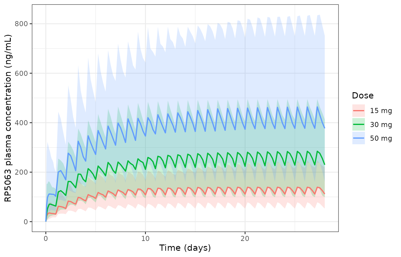

Simulated RP5063 plasma concentration over the 28-day regimen (median and 90% prediction interval). Replicates the shape of Figure 3 of Cantillon 2018.

Steady state is approached over roughly the first 5 days, consistent with the phase 1 multiple-dose observation quoted in Sect. 1 (“steady state was approached after 120 h of daily dosing”).

Dose linearity

Sect. 3.3 reports pairwise t-tests that failed to reject equality of Cl/F across the three dose arms, i.e. linear PK over 15-50 mg. The model has no non-linear term, so exposure must be exactly dose-proportional.

Proportionality is a property of each individual, so it is asserted on the typical-value solve, where the three arms share one parameter vector. (Medians across three independently drawn arms are not exactly proportional, because each arm draws its own BMI and random effects.)

lin_typ <- tibble::tibble(treatment = c("15 mg", "30 mg", "50 mg"),
                          dose_mg = c(15, 30, 50), BMI = 23.01,
                          REGION_MOLDOVA = 0) |>
  mutate(id = row_number())

sim_lin <- rxode2::rxSolve(mod_typ, make_events(lin_typ, c(0, 672), n_doses = 28),
                           keep = "treatment") |>
  as.data.frame() |>
  filter(time == 672) |>
  left_join(lin_typ |> select(id, dose_mg), by = "id") |>
  transmute(treatment, `Dose (mg)` = dose_mg,
            `Cumulative AUC (ug*h/mL)` = auc_central,
            `AUC per mg` = auc_central / dose_mg)
#> ℹ omega/sigma items treated as zero: 'etalcl', 'etalvc', 'etalka', 'etae0', 'etaemax', 'etalauc50'
#> Warning: multi-subject simulation without without 'omega'

knitr::kable(sim_lin, digits = 4,
             caption = "Typical-value cumulative AUC at day 28 scales exactly with dose.")

Typical-value cumulative AUC at day 28 scales exactly with dose.

treatment	Dose (mg)	Cumulative AUC (ug*h/mL)	AUC per mg
15 mg	15	75.4252	5.0283
30 mg	30	150.8504	5.0283
50 mg	50	251.4173	5.0283

stopifnot(
  # Deterministic consequence of a linear model: solver noise only.
  diff(range(sim_lin$`AUC per mg`)) / mean(sim_lin$`AUC per mg`) < 1e-6
)

In the stochastic cohort the per-arm medians are close but not identical, reflecting the independent covariate and random-effect draws in each arm:

sim_md |>
  filter(time == max(time)) |>
  group_by(treatment) |>
  summarise(`Median cumulative AUC (ug*h/mL)` = median(auc_central),
            .groups = "drop") |>
  mutate(`Dose (mg)` = c(15, 30, 50),
         `AUC per mg` = `Median cumulative AUC (ug*h/mL)` / `Dose (mg)`) |>
  knitr::kable(digits = 3,
               caption = "Stochastic cohort medians (descriptive).")

Stochastic cohort medians (descriptive).

treatment	Median cumulative AUC (ug*h/mL)	Dose (mg)	AUC per mg
15 mg	80.541	15	5.369
30 mg	157.468	30	5.249
50 mg	251.025	50	5.020

Body mass index affects volume but not average steady-state exposure

Sect. 4 makes an explicit, directly testable claim:

Since BMI only affected volume of distribution, this covariate should not affect the average steady-state plasma levels of RP5063, since clearance did not change.

bmi_grid <- tibble::tibble(BMI = c(18, 23.01, 30, 35)) |>
  mutate(id = row_number(), treatment = "30 mg", dose_mg = 30, REGION_MOLDOVA = 0)

ev_bmi <- make_events(bmi_grid, seq(0, 672, by = 1), n_doses = 28)
sim_bmi <- rxode2::rxSolve(mod_typ, ev_bmi, keep = c("BMI")) |> as.data.frame()
#> ℹ omega/sigma items treated as zero: 'etalcl', 'etalvc', 'etalka', 'etae0', 'etaemax', 'etalauc50'
#> Warning: multi-subject simulation without without 'omega'

bmi_tab <- sim_bmi |>
  filter(time >= 648) |>
  group_by(BMI) |>
  summarise(`Cavg day 28 (ng/mL)` = mean(Cc),
            `Cmax day 28 (ng/mL)` = max(Cc), .groups = "drop") |>
  mutate(`Vc/F (L)` = 328 * (BMI / 23.01)^0.90,
         `t1/2 (h)` = log(2) * `Vc/F (L)` / 5.11) |>
  select(BMI, `Vc/F (L)`, `t1/2 (h)`, `Cavg day 28 (ng/mL)`, `Cmax day 28 (ng/mL)`)

knitr::kable(bmi_tab, digits = 2,
             caption = "BMI moves Vc/F and half-life substantially, but leaves average steady-state concentration unchanged (Cantillon 2018 Sect. 4).")

BMI moves Vc/F and half-life substantially, but leaves average steady-state concentration unchanged (Cantillon 2018 Sect. 4).

BMI	Vc/F (L)	t1/2 (h)	Cavg day 28 (ng/mL)	Cmax day 28 (ng/mL)
18.00	262.96	35.67	243.02	276.46
23.01	328.00	44.49	243.32	270.01
30.00	416.45	56.49	243.52	264.45
35.00	478.42	64.90	243.53	261.70

stopifnot(
  # Volume nearly doubles across the BMI range examined...
  max(bmi_tab$`Vc/F (L)`) / min(bmi_tab$`Vc/F (L)`) > 1.7,
  # ...while average steady-state concentration moves by well under 1%.
  diff(range(bmi_tab$`Cavg day 28 (ng/mL)`)) /
    mean(bmi_tab$`Cavg day 28 (ng/mL)`) < 0.01
)

PKNCA validation

The paper reports one NCA-comparable quantity, the calculated terminal half-life of 44.5 h. The typical-value (inter-individual variability zeroed) single-dose profile is used for the gate, because the model’s IIV on ka (variance 2.09, i.e. a 266% CV) puts a meaningful fraction of simulated subjects into flip-flop kinetics, where a terminal-slope half-life reflects absorption rather than elimination. The stochastic cohort is reported descriptively alongside.

typ <- tibble::tibble(
  treatment = c("15 mg", "30 mg", "50 mg"), dose_mg = c(15, 30, 50),
  BMI = 23.01, REGION_MOLDOVA = 0
) |> mutate(id = row_number())

times_sd <- c(0, 0.5, 1, 2, 3, 4, 6, 8, 10, 12, 16, 20, 24, 30, 36, 48, 60, 72,
              96, 120, 168, 216, 264, 336, 408, 504)
ev_sd <- make_events(typ, times_sd, n_doses = 1)

sim_sd <- rxode2::rxSolve(mod_typ, ev_sd, keep = c("treatment")) |>
  as.data.frame()

conc_sd <- sim_sd |>
  filter(!is.na(Cc)) |>
  select(id, time, Cc, treatment)
conc_sd <- bind_rows(
  conc_sd,
  conc_sd |> distinct(id, treatment) |> mutate(time = 0, Cc = 0)
) |>
  distinct(id, treatment, time, .keep_all = TRUE) |>
  arrange(id, treatment, time)

dose_sd <- ev_sd |> filter(evid == 1) |> select(id, time, amt, treatment)

conc_obj <- PKNCA::PKNCAconc(conc_sd, Cc ~ time | treatment + id,
                             concu = "ng/mL", timeu = "h")
dose_obj <- PKNCA::PKNCAdose(dose_sd, amt ~ time | treatment + id, doseu = "mg")

intervals <- data.frame(start = 0, end = Inf, cmax = TRUE, tmax = TRUE,
                        aucinf.obs = TRUE, half.life = TRUE, lambda.z = TRUE)

nca_typ <- PKNCA::pk.nca(PKNCA::PKNCAdata(conc_obj, dose_obj,
                                          intervals = intervals))

The reference column below carries the paper’s calculated half-life of 44.5 h (Sect. 3.3 and Key Points) and the AUC0-inf implied by the paper’s own Cl/F of 5.11 L/h (Table 2), i.e. dose / (Cl/F), converted to ng*h/mL. The latter is derived from Table 2 rather than tabulated as an NCA result in the paper.

published <- tibble::tibble(
  treatment = c("15 mg", "30 mg", "50 mg"),
  aucinf.obs = c(15, 30, 50) / 5.11 * 1000,
  half.life = 44.5
)

cmp <- nlmixr2lib::ncaComparisonTable(
  simulated = nca_typ,
  reference = published,
  by = "treatment",
  units = c(aucinf.obs = "ng*h/mL", half.life = "h"),
  tolerance_pct = 20
)

knitr::kable(cmp, caption = paste(
  "Simulated (typical-value) vs. published NCA.",
  "* marks rows differing from the reference by more than 20%."
))

Simulated (typical-value) vs. published NCA. * marks rows differing from the reference by more than 20%.

NCA parameter	treatment	Reference	Simulated	% diff
AUC0-∞ (obs) (ng*h/mL)	15 mg	2940	2930	-0.1%
AUC0-∞ (obs) (ng*h/mL)	30 mg	5870	5870	-0.1%
AUC0-∞ (obs) (ng*h/mL)	50 mg	9780	9780	-0.1%
t½ (h)	15 mg	44.5	44.5	+0.0%
t½ (h)	30 mg	44.5	44.5	+0.0%
t½ (h)	50 mg	44.5	44.5	+0.0%

nca_wide <- as.data.frame(nca_typ$result) |>
  filter(PPTESTCD %in% c("half.life", "aucinf.obs")) |>
  tidyr::pivot_wider(id_cols = treatment, names_from = PPTESTCD,
                     values_from = PPORRES)

stopifnot(
  # Deterministic typical-value profile against the paper's closed-form
  # half-life, so a tight bound is appropriate here.
  all(abs(nca_wide$half.life - 44.5) < 0.5),
  # AUC0-inf must recover dose / (Cl/F) to within trapezoidal error.
  all(abs(nca_wide$aucinf.obs / (c(15, 30, 50) / 5.11 * 1000) - 1) < 0.02)
)

rxode2::rxSetSeed(20260919)

ev_sd_pop <- make_events(cohort, times_sd, n_doses = 1)
sim_sd_pop <- rxode2::rxSolve(mod, ev_sd_pop, keep = c("treatment")) |>
  as.data.frame()

conc_pop <- sim_sd_pop |> filter(!is.na(Cc)) |> select(id, time, Cc, treatment)
conc_pop <- bind_rows(
  conc_pop,
  conc_pop |> distinct(id, treatment) |> mutate(time = 0, Cc = 0)
) |>
  distinct(id, treatment, time, .keep_all = TRUE) |>
  arrange(id, treatment, time)

nca_pop <- PKNCA::pk.nca(PKNCA::PKNCAdata(
  PKNCA::PKNCAconc(conc_pop, Cc ~ time | treatment + id,
                   concu = "ng/mL", timeu = "h"),
  PKNCA::PKNCAdose(ev_sd_pop |> filter(evid == 1) |>
                     select(id, time, amt, treatment),
                   amt ~ time | treatment + id, doseu = "mg"),
  intervals = intervals
))

as.data.frame(nca_pop$result) |>
  filter(PPTESTCD %in% c("cmax", "tmax", "half.life", "aucinf.obs")) |>
  group_by(treatment, PPTESTCD) |>
  summarise(Median = median(PPORRES, na.rm = TRUE),
            `P10` = quantile(PPORRES, 0.10, na.rm = TRUE),
            `P90` = quantile(PPORRES, 0.90, na.rm = TRUE), .groups = "drop") |>
  mutate(Parameter = nlmixr2lib::ncaParamLabel(PPTESTCD)) |>
  select(Parameter, treatment, Median, P10, P90) |>
  knitr::kable(digits = 2, caption = paste(
    "Stochastic cohort NCA (descriptive). The wide half-life spread is driven",
    "by the 266% CV on ka, which pushes slowly-absorbing subjects into",
    "flip-flop kinetics."
  ))

Stochastic cohort NCA (descriptive). The wide half-life spread is driven by the 266% CV on ka, which pushes slowly-absorbing subjects into flip-flop kinetics.

Parameter	treatment	Median	P10	P90
AUC0-∞ (obs)	15 mg	3202.63	1842.05	5149.44
Cmax	15 mg	37.80	22.29	69.38
t½	15 mg	42.35	20.24	108.97
Tmax	15 mg	10.00	2.00	30.00
AUC0-∞ (obs)	30 mg	6381.42	3367.82	10398.88
Cmax	30 mg	77.06	31.99	143.17
t½	30 mg	47.90	21.24	97.83
Tmax	30 mg	10.00	2.00	30.60
AUC0-∞ (obs)	50 mg	10153.13	6405.59	16348.11
Cmax	50 mg	123.52	65.20	282.08
t½	50 mg	47.90	20.87	108.21
Tmax	50 mg	8.00	2.90	24.00

Pharmacodynamics: PANSS versus cumulative exposure

Model selection (Sect. 3.4) found cumulative AUC to be the best of the four candidate predictors (instantaneous concentration, effect-compartment concentration, daily average concentration, cumulative AUC), and a placebo term made the fit worse and was dropped.

auc_grid <- tibble::tibble(auc = seq(0, 400, length.out = 200)) |>
  mutate(PANSS = 87.3 + (-31.6) * auc / (auc + 89.6))

ggplot(auc_grid, aes(auc, PANSS)) +
  geom_line(linewidth = 0.8) +
  geom_vline(xintercept = 89.6, linetype = "dotted") +
  annotate("text", x = 89.6, y = 86, label = "AUC50 = 89.6", hjust = -0.05,
           size = 3) +
  labs(x = "Cumulative AUC (ug*h/mL)", y = "Total PANSS") +
  theme_bw()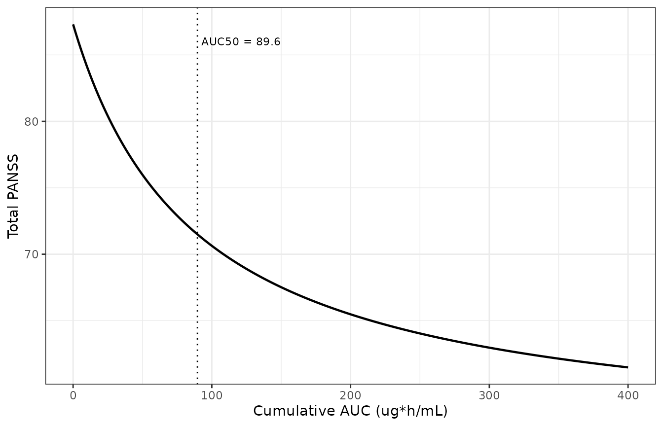

Predicted total PANSS as a function of cumulative RP5063 AUC. Replicates the model fit line of Figure 4 of Cantillon 2018.

Dose-response relationship (Figure 6)

Figure 6 of the paper plots predicted total PANSS against daily dose, with a solid line for the base model and a dashed line for the model carrying the geographic-site effect on Emax. Both are reproduced by solving the typical-value model for 28 days over a dose grid.

dose_grid <- tidyr::expand_grid(
  dose_mg = seq(2.5, 60, by = 2.5),
  REGION_MOLDOVA = c(0, 1)
) |>
  mutate(id = row_number(), BMI = 23.01,
         treatment = ifelse(REGION_MOLDOVA == 1, "With Moldova site effect",
                            "Base model"))

ev_dr <- make_events(dose_grid, c(0, 672), n_doses = 28)
sim_dr <- rxode2::rxSolve(mod_typ, ev_dr,
                          keep = c("treatment", "REGION_MOLDOVA")) |>
  as.data.frame() |>
  filter(time == 672) |>
  left_join(dose_grid |> select(id, dose_mg), by = "id")

ggplot(sim_dr, aes(dose_mg, PANSS, linetype = treatment)) +
  geom_line(linewidth = 0.8) +
  geom_hline(yintercept = 87.3, colour = "grey60", linetype = "dotted") +
  annotate("rect", xmin = 5, xmax = 30, ymin = -Inf, ymax = Inf, alpha = 0.08,
           fill = "steelblue") +
  labs(x = "Daily dose (mg)", y = "Predicted total PANSS at day 28",
       linetype = NULL,
       caption = "Shaded band: the 5-30 mg range the paper identifies as clinically relevant.") +
  theme_bw() +
  theme(legend.position = "bottom")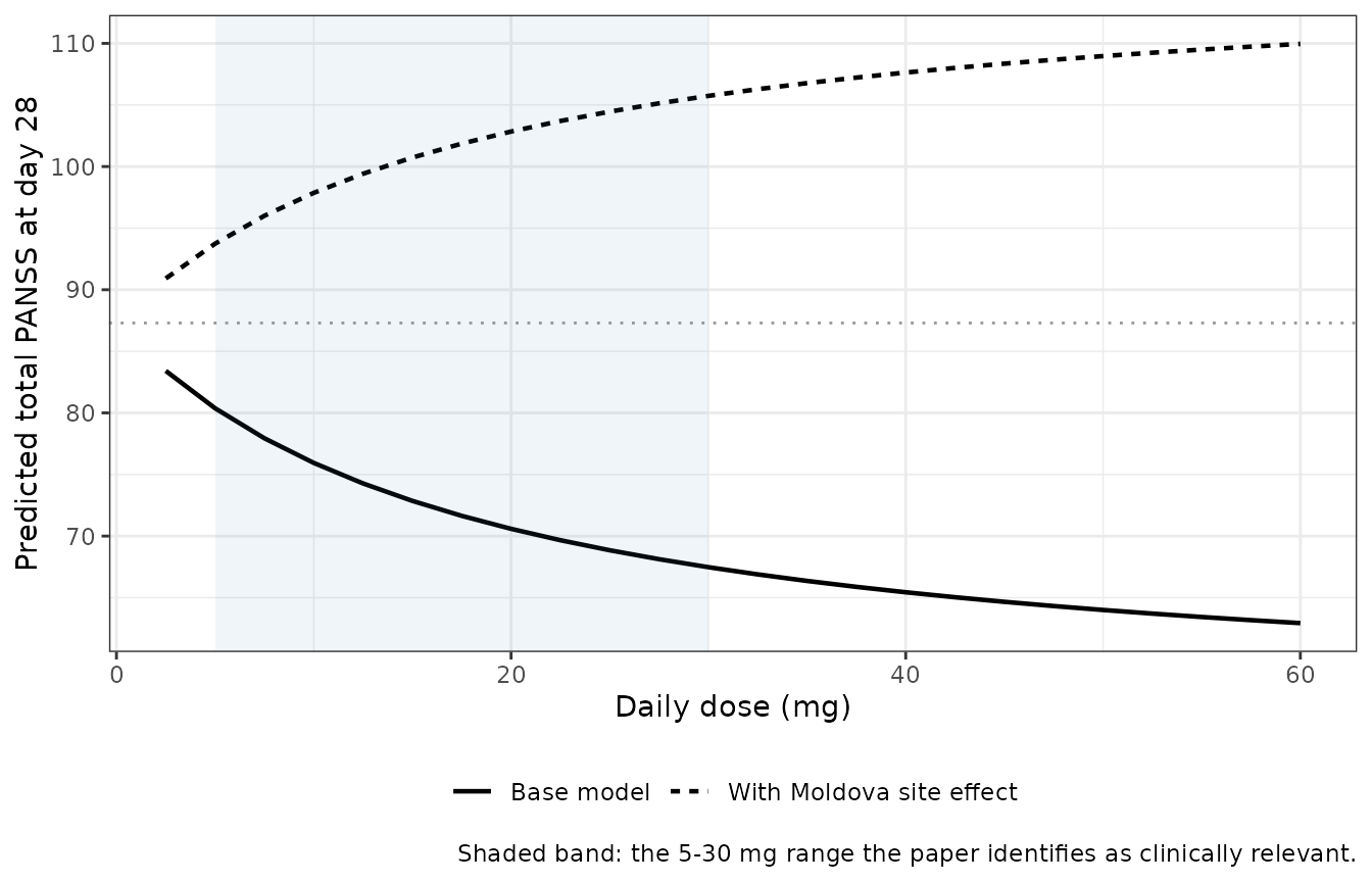

Predicted total PANSS at day 28 versus daily dose, with and without the Moldova study-site effect on Emax. Replicates Figure 6 of Cantillon 2018.

The paper concludes (Sect. 3.4, Sect. 5) that “daily doses between 5 and 30 mg should adequately describe a clinically relevant dose/efficacy relationship”. The simulated curve reproduces that: most of the attainable PANSS improvement is realised by 30 mg, and the curve flattens above it.

base_dr <- sim_dr |> filter(REGION_MOLDOVA == 0) |> arrange(dose_mg)
get_change <- function(d) {
  base_dr$PANSS[which.min(abs(base_dr$dose_mg - d))] - 87.3
}

dr_tab <- tibble::tibble(
  `Daily dose (mg)` = c(5, 15, 30, 50),
  `PANSS change at day 28 (pu)` = round(vapply(c(5, 15, 30, 50), get_change, 0), 2)
)
knitr::kable(dr_tab, caption = "Predicted PANSS change from baseline at day 28.")

Predicted PANSS change from baseline at day 28.

Daily dose (mg)	PANSS change at day 28 (pu)
5	-6.92
15	-14.44
30	-19.82
50	-23.30

stopifnot(
  # Monotonically increasing improvement with dose.
  all(diff(base_dr$PANSS) < 0),
  # The 5-30 mg window captures most of the change realised by 50 mg. The
  # changes are negative (PANSS improves by falling), so compare magnitudes.
  abs(get_change(30) - get_change(5)) >
    2 * abs(get_change(50) - get_change(30)),
  # ...and the Moldova arm moves PANSS in the opposite direction.
  all(sim_dr$PANSS[sim_dr$REGION_MOLDOVA == 1 & sim_dr$dose_mg > 5] > 87.3)
)

Comparison with the observed trial arm means

The REFRESH primary-endpoint analysis (quoted in Sect. 1) reported mean (SE) PANSS changes of -20.23 (2.65), -15.42 (2.04) and -19.21 (2.39) for the 15, 30 and 50 mg arms.

sim_panss <- sim_md |>
  filter(time == 672) |>
  group_by(treatment) |>
  summarise(`Model median change (pu)` = round(median(PANSS) - 87.3, 2),
            .groups = "drop") |>
  mutate(`Observed change (pu)` = c(-20.23, -15.42, -19.21),
         `Observed SE` = c(2.65, 2.04, 2.39))

knitr::kable(sim_panss, caption = paste(
  "Model-predicted vs. observed PANSS change at day 28. The Emax model is",
  "monotone in dose by construction and does not reproduce the non-monotone",
  "ordering of the observed arm means."
))

Model-predicted vs. observed PANSS change at day 28. The Emax model is monotone in dose by construction and does not reproduce the non-monotone ordering of the observed arm means.

treatment	Model median change (pu)	Observed change (pu)	Observed SE
15 mg	-15.31	-20.23	2.65
30 mg	-18.37	-15.42	2.04
50 mg	-17.47	-19.21	2.39

The model is monotone in dose, whereas the observed arm means are not (the 30 mg arm improved least). This is a property of the published model, not of the encoding: Cantillon 2018 fitted a single Emax curve through all subject-level PANSS-versus-exposure pairs rather than to the arm means, and Figures 4 and 5 show the corresponding scatter. No parameter has been adjusted to improve this comparison.

Assumptions and deviations

• Variance versus standard deviation in Tables 2 and 3. The tables label their random-effect rows “Var(g1)”, “Cov(g1, g2)” and “sigma_1^2” / “sigma^2” (i.e. sigma^2), so the tabulated numbers are read as variances. Three independent checks agree:
  1. the covariance row implies a correlation of 0.04 / sqrt(0.16 * 0.28) = 0.19 under the variance reading, against 0.89 under a standard-deviation reading;
  2. Var(eta E0) = 164 gives an E0 standard deviation of 12.8 PANSS units, matching the observed per-arm baseline PANSS SDs of 13.3 / 13.4 / 14.9 in Table 1, whereas a standard-deviation reading would place 164 PANSS units of spread on a scale bounded at 30-210;
  3. the empirical-Bayes Cl/F of Sect. 3.3, 5.17 +/- 0.24 L/h over 58 subjects, is a mean +/- standard error, implying an EBE standard deviation of 1.83 L/h and a CV of 35% - consistent with the 42% CV of Var = 0.16 after shrinkage, but impossible under the 16% CV of a standard-deviation reading, since empirical-Bayes spread cannot exceed the true IIV.
• Errata: the base-model variability percentages in Sect. 3.2 are inconsistent with Table 2. Sect. 3.2 reports base-model inter-subject CVs of “14.90 and 21.40% for Cl/F and Vc/F” and an intra-subject CV of “approximately 8.0%”. Under the variance reading adopted here the final-model values are 42%, 57% and 26%. The Sect. 3.2 figures are also internally suspicious: 14.90 is the same number as the Vc/F standard error quoted in the immediately preceding sentence. Because a covariate addition cannot inflate an IIV variance sevenfold, and because check (c) above rules the small values out directly, Table 2 is used. A reader who preferred the Sect. 3.2 reading would set etalcl ~ 0.0222, etalvc ~ 0.0459 and propSd <- 0.08.
• Supplementary appendices are not on disk. Appendices A-D (sampling-time blocks, bioanalytical method, PD covariate stepwise table, concomitant medication list) were not available. None contains a parameter used by the model; the covariate-screen results they support are documented in covariatesDataExcluded.
• ka is poorly identified. Table 2 gives Var(g3) = 2.09 with a standard error of 6.63, i.e. a relative standard error above 300%, and the point estimate of ka itself has an RSE of 40%. Sect. 4 attributes this to the absence of early post-dose sampling. Simulated single-subject absorption profiles are correspondingly variable and a small fraction show flip-flop kinetics; this is faithful to the published model, not an encoding artefact.
• Cumulative, not steady-state, AUC. The auc_central state integrates concentration from the first dose and therefore keeps rising for the whole 28-day course. This is the paper’s Eq. 11 predictor. It is not a dosing-interval AUC, and AUC50 = 89.6 ug*h/mL is not comparable to a steady-state AUC0-24 for this drug (which is about 3-10 ug*h/mL).
• The Moldova site effect is a measurement artefact, per the authors. Sect. 3.4 and Sect. 4 report that the site influenced only the PANSS endpoint, not the PK, and describe the data as an outlier. It is encoded because it is in the final model, but REGION_MOLDOVA = 0 reproduces the paper’s base dose-response relationship.
• No placebo term. Eq. 13’s alpha * t placebo component was tested and rejected (the objective function increased); no alpha estimate is reported, so none is encoded.
• No bioavailability parameter. Cl/F and Vc/F are apparent oral values throughout; the paper reports no F and no intravenous reference arm, so absolute volume and clearance are not identifiable.
• Drug naming. The paper calls the compound RP5063 throughout; the model file uses the INN, brilaroxazine, per the library’s generic-name convention.
• Two-compartment structure not carried. Sect. 3.2 reports that a two-compartment fit produced parameter correlations above 0.95 and no computable standard errors, so the authors selected the one-compartment model; Sect. 4 notes the distribution phase carries under 10% of total AUC. Only the published one-compartment model is encoded.

Session info

sessionInfo()
#> R version 4.6.1 (2026-06-24)
#> Platform: x86_64-pc-linux-gnu
#> Running under: Ubuntu 24.04.5 LTS
#> 
#> Matrix products: default
#> BLAS:   /usr/lib/x86_64-linux-gnu/openblas-pthread/libblas.so.3 
#> LAPACK: /usr/lib/x86_64-linux-gnu/openblas-pthread/libopenblasp-r0.3.26.so;  LAPACK version 3.12.0
#> 
#> locale:
#>  [1] LC_CTYPE=C.UTF-8       LC_NUMERIC=C           LC_TIME=C.UTF-8       
#>  [4] LC_COLLATE=C.UTF-8     LC_MONETARY=C.UTF-8    LC_MESSAGES=C.UTF-8   
#>  [7] LC_PAPER=C.UTF-8       LC_NAME=C              LC_ADDRESS=C          
#> [10] LC_TELEPHONE=C         LC_MEASUREMENT=C.UTF-8 LC_IDENTIFICATION=C   
#> 
#> time zone: UTC
#> tzcode source: system (glibc)
#> 
#> attached base packages:
#> [1] stats     graphics  grDevices utils     datasets  methods   base     
#> 
#> other attached packages:
#> [1] ggplot2_4.0.3         dplyr_1.2.1           PKNCA_0.12.1         
#> [4] rxode2_5.1.8          nlmixr2lib_0.3.2.9000
#> 
#> loaded via a namespace (and not attached):
#>  [1] gtable_0.3.6        xfun_0.61           bslib_0.12.0       
#>  [4] rxode2lincmt_0.1.0  lattice_0.22-9      vctrs_0.7.3        
#>  [7] tools_4.6.1         generics_0.1.4      parallel_4.6.1     
#> [10] tibble_3.3.1        symengine_0.2.13    pkgconfig_2.0.3    
#> [13] data.table_1.18.6.1 checkmate_2.3.4     RColorBrewer_1.1-3 
#> [16] S7_0.2.2            desc_1.4.3          lifecycle_1.0.5    
#> [19] compiler_4.6.1      farver_2.1.2        textshaping_1.0.5  
#> [22] fontawesome_0.5.3   htmltools_0.5.9     sys_3.4.3          
#> [25] sass_0.4.10         yaml_2.3.12         pillar_1.11.1      
#> [28] pkgdown_2.2.1       crayon_1.5.3        jquerylib_0.1.4    
#> [31] whisker_0.4.1       tidyr_1.3.2         openssl_2.4.2      
#> [34] cachem_1.1.0        nlme_3.1-169        tidyselect_1.2.1   
#> [37] digest_0.6.39       lotri_1.0.5         purrr_1.2.2        
#> [40] labeling_0.4.3      rxode2ll_2.0.18     fastmap_1.2.0      
#> [43] grid_4.6.1          cli_3.6.6           dparser_1.3.1-13   
#> [46] magrittr_2.0.5      withr_3.0.3         scales_1.4.0       
#> [49] backports_1.5.1     rmarkdown_2.32      otel_0.2.0         
#> [52] askpass_1.2.1       ragg_1.5.2          memoise_2.0.1      
#> [55] evaluate_1.0.5      knitr_1.52          rex_1.2.2          
#> [58] PreciseSums_0.7     rlang_1.3.0         downlit_0.4.5      
#> [61] Rcpp_1.1.2          glue_1.8.1          xml2_1.6.0         
#> [64] jsonlite_2.0.0      R6_2.6.1            systemfonts_1.3.2  
#> [67] fs_2.1.0