Ertugliflozin in select ethnic populations (Fediuk 2021b)
Source:vignettes/articles/Fediuk_2021b_ertugliflozin_ethnicity.Rmd
Fediuk_2021b_ertugliflozin_ethnicity.RmdModel and source
- Citation: Fediuk DJ, Sahasrabudhe V, Dawra VK, Zhou S, Sweeney K (2021). Population Pharmacokinetic Analyses of Ertugliflozin in Select Ethnic Populations. Clinical Pharmacology in Drug Development 10(11):1297-1306. doi:10.1002/cpdd.970. Absorption covariate parameterization from Fediuk DJ et al. (2021) Clin Pharmacol Drug Dev 10(7):696-706, doi:10.1002/cpdd.885 (Supplementary Appendix Equations 7-8).
- Article: https://doi.org/10.1002/cpdd.970 (open access; PMC9291861)
- Supplement: Supporting Information file s001 holds the two added studies (Table S1), their sampling schemes (Table S2) and the final covariate equations of both analyses (Table S3).
- Parent analysis: the structural model, the eGFR definition and the
food parameterization on ka and F1 come from Fediuk 2021 (https://doi.org/10.1002/cpdd.885), packaged as
Fediuk_2021_ertugliflozin.
Fediuk 2021b ran two independent population PK analyses of the oral SGLT2 inhibitor ertugliflozin to support registration in East/Southeast Asia and in China. Both start from the two-compartment model of the parent analysis (lag time, first-order absorption and elimination) and re-estimate the full covariate model with a different ethnicity covariate:
-
Analysis 1 (data set 1) compares East/Southeast
(E/SE) Asian with non-E/SE Asian subjects. Packaged as
Fediuk_2021b_ertugliflozin_esea. -
Analysis 2 (data set 2) compares Asian subjects
from mainland China and Asian subjects from the rest of the world (ROW)
with non-Asian subjects. Packaged as
Fediuk_2021b_ertugliflozin_china.
mod_esea <- readModelDb("Fediuk_2021b_ertugliflozin_esea")
mod_china <- readModelDb("Fediuk_2021b_ertugliflozin_china")
mod_esea_typ <- rxode2::zeroRe(mod_esea)
#> ℹ parameter labels from comments will be replaced by 'label()'
#> Warning: No sigma parameters in the model
mod_china_typ <- rxode2::zeroRe(mod_china)
#> ℹ parameter labels from comments will be replaced by 'label()'
#> Warning: No sigma parameters in the model
Population
Data set 1 is the parent analysis data set: 13,692 concentrations from 2276 subjects in 15 phase 1-3 studies, 91.6% with type 2 diabetes mellitus (T2DM). Subjects counted as E/SE Asian (N = 154, 6.8%) were the Japanese subjects of a phase 1 PK/pharmacodynamic study and the self-reported Asian subjects of the phase 2/3 studies enrolled in Hong Kong, the Republic of Korea, Malaysia, the Philippines, Taiwan and Thailand. Asian subjects enrolled at US or European sites counted as non-E/SE Asian (N = 2122).
Data set 2 adds a phase 1 study in healthy Chinese subjects (I-10, N = 16) and a phase 3 study in Asian patients with T2DM (III-5, N = 330) (Table S1), giving 16,018 concentrations from 2620 subjects (92.1% T2DM): 277 Asian subjects from mainland China (10.6%), 382 Asian subjects from the ROW (14.6%) and 1961 non-Asian subjects (74.8%).
Demographics were similar across the groups except body weight, which was lower in every Asian group (Table 1):
| Group | N | Weight mean (SD), kg | Age mean (SD), y | eGFR mean (SD), mL/min/1.73 m^2 | Female | T2DM |
|---|---|---|---|---|---|---|
| Data set 1, E/SE Asian | 154 | 69.7 (14.6) | 54.1 (10.4) | 85.3 (25.3) | 48.7% | 92.2% |
| Data set 1, non-E/SE Asian | 2122 | 88.2 (19.4) | 55.8 (11.7) | 85.9 (24.3) | 43.1% | 91.5% |
| Data set 2, Asian from mainland China | 277 | 70.5 (10.7) | 54.5 (11.0) | 103 (20.9) | 43.0% | 94.2% |
| Data set 2, Asian from the ROW | 382 | 72.8 (15.4) | 54.9 (10.1) | 87.4 (21.9) | 40.8% | 96.1% |
| Data set 2, non-Asian | 1961 | 89.1 (19.4) | 55.8 (11.8) | 85.7 (24.6) | 44.0% | 91.0% |
mod_china()$population[c("n_subjects", "n_studies", "race_ethnicity")]
#> $n_subjects
#> [1] 2620
#>
#> $n_studies
#> [1] 17
#>
#> $race_ethnicity
#> Asian from mainland China  Asian from rest of world                 non-Asian
#>                      10.6                      14.6                      74.8
Source trace
Every ini() value carries an in-file comment pointing to
Table 2 of Fediuk 2021b. The table collects them for both models.
| Parameter | Data set 1 (_esea) |
Data set 2 (_china) |
Source location |
|---|---|---|---|
lcl (CL/F, L/h) |
log(11.9) | log(11.8) | Table 2 |
lvc (Vc/F, L) |
log(6.51) | log(5.23) | Table 2 |
lvp (Vp/F, L) |
log(107) | log(113) | Table 2 |
lq (Q/F, L/h) |
log(7.76) | log(7.17) | Table 2 |
lka (ka fasted, 1/h) |
log(0.329) | log(0.323) | Table 2 |
ltlag (lag time, h) |
log(0.226) | log(0.227) | Table 2 |
lfdepot (F1 fasted) |
fixed(log(1)) | fixed(log(1)) | Table 2, 1.00 (fixed) |
e_wt_cl_q / e_wt_vc_vp
|
fixed(0.75) / fixed(1) | fixed(0.75) / fixed(1) | Table 2 (fixed) rows; Table S3 |
e_crcl_cl |
0.458 | 0.449 | Table 2, CL/F ‘Effect of eGFR’ |
e_dis_diab_cl |
0.921 | 0.856 | Table 2, CL/F ‘Effect of T2DM patient status’ |
e_sexf_cl |
0.960 | 0.970 | Table 2, CL/F ‘Effect of female sex’ |
e_asian_esea_cl |
1.17 | n/a | Table 2, CL/F ‘Effect of E/SE Asian ethnicity’ |
e_asian_china_cl / e_asian_row_cl
|
n/a | 1.04 / 1.08 | Table 2, CL/F Asian rows |
e_age_vc |
-0.192 | -0.603 | Table 2, Vc/F ‘Effect of age’ |
e_sexf_vc |
1.46 | 1.66 | Table 2, Vc/F ‘Effect of female sex’ |
e_asian_esea_vc |
2.48 | n/a | Table 2, Vc/F ‘Effect of E/SE Asian ethnicity’ |
e_asian_china_vc / e_asian_row_vc
|
n/a | 1.44 / 2.15 | Table 2, Vc/F Asian rows |
e_fed_ka / e_fed_missing_ka
|
0.725 / 0.654 | 0.639 / 0.796 | Table 2, ka food rows |
e_fed_fdepot / e_fed_missing_fdepot
|
0.0702 / 0.0681 | 0.157 / 0.148 | Table 2, F1 food rows |
etalcl (variance) |
0.101 | 0.0999 | Table 2 omega^2 CL/F; 31.8% / 31.6% CV in Results |
expSdPh1 / expSdPh23
|
0.389 / 0.837 | 0.486 / 0.831 | Table 2 residual rows; Results percentages |
| CL/F, Vc/F, Vp/F, Q/F covariate equations | E/SE Asian indicator EASIA | RACE2 / RACE3 | Table S3 |
| Reference subject and eGFR cap at 120 | 65 y, healthy, male, 85 kg, eGFR 90, fasted | same, non-Asian | Methods, Data Set 1 / Data Set 2 |
ka and F1 food equations,
F1 = 1 - FED*theta - FED_MISSING*theta
|
parent analysis | parent analysis | Fediuk 2021 Supplementary Appendix Equations 7-8 |
Cc ~ lnorm() (additive on log concentration) |
parent analysis | parent analysis | Fediuk 2021 Supplementary Appendix Equation 4 |
Ethnicity encoding
Table S3 uses one indicator in data set 1 (EASIA) and two in data set 2 (RACE2, RACE3). Both are combinations of self-reported Asian ethnicity and where the subject was enrolled, so the packaged models build them from the canonical race and region columns:
- data set 1:
EASIA = RACE_ASIAN * (REGION_EASTASIA + REGION_SOUTHEASTASIA) - data set 2:
RACE2 = RACE_ASIAN * REGION_CHINA,RACE3 = RACE_ASIAN * (1 - REGION_CHINA)
The chunk below confirms that the encoding reproduces the paper’s categories: an Asian subject enrolled in the US is non-E/SE Asian in data set 1, and a non-Asian subject enrolled in China is in the non-Asian reference of data set 2.
ref_cov <- tibble(
  WT = 85, AGE = 65, CRCL = 90, DIS_DIAB = 0, SEXF = 0,
  RACE_ASIAN = 0, REGION_EASTASIA = 0, REGION_SOUTHEASTASIA = 0,
  REGION_CHINA = 0,
  FED = 0, FED_MISSING = 0, STUDY_PHASE2 = 0, STUDY_PHASE3 = 0
)

# One dose and one observation per scenario return the typical cl, vc and
# fdepot as algebraic outputs.
typical_par <- function(mod, scen) {
  scen <- scen |> mutate(id = row_number())
  ev <- bind_rows(
    scen |> mutate(time = 0, evid = 1L, amt = 15, cmt = "depot"),
    scen |> mutate(time = 1, evid = 0L, amt = 0, cmt = "central")
  ) |>
    arrange(id, time)
  rxode2::rxSolve(mod, ev, keep = "scenario", returnType = "data.frame") |>
    select(scenario, cl, vc, fdepot)
}

scen_esea <- bind_rows(
  ref_cov |> mutate(scenario = "Reference (non-E/SE Asian)"),
  ref_cov |> mutate(scenario = "Asian, Korea site", RACE_ASIAN = 1, REGION_EASTASIA = 1),
  ref_cov |> mutate(scenario = "Asian, Thailand site", RACE_ASIAN = 1, REGION_SOUTHEASTASIA = 1),
  ref_cov |> mutate(scenario = "Asian, US site", RACE_ASIAN = 1),
  ref_cov |> mutate(scenario = "Non-Asian, Korea site", REGION_EASTASIA = 1)
)
scen_china <- bind_rows(
  ref_cov |> mutate(scenario = "Reference (non-Asian)"),
  ref_cov |> mutate(scenario = "Asian, mainland China", RACE_ASIAN = 1, REGION_CHINA = 1),
  ref_cov |> mutate(scenario = "Asian, rest of world", RACE_ASIAN = 1),
  ref_cov |> mutate(scenario = "Non-Asian, China site", REGION_CHINA = 1)
)

typ_esea <- typical_par(mod_esea_typ, scen_esea) |>
  mutate(model = "Data set 1", cl_ratio = cl / cl[1], vc_ratio = vc / vc[1])
#> ℹ omega/sigma items treated as zero: 'etalcl'
#> Warning: multi-subject simulation without without 'omega'
typ_china <- typical_par(mod_china_typ, scen_china) |>
  mutate(model = "Data set 2", cl_ratio = cl / cl[1], vc_ratio = vc / vc[1])
#> ℹ omega/sigma items treated as zero: 'etalcl'
#> Warning: multi-subject simulation without without 'omega'
typ <- bind_rows(typ_esea, typ_china)

typ |>
  select(model, scenario, cl, vc, cl_ratio, vc_ratio) |>
  rename(
    "Model" = model, "Scenario" = scenario, "CL/F (L/h)" = cl,
    "Vc/F (L)" = vc, "CL/F ratio" = cl_ratio, "Vc/F ratio" = vc_ratio
  ) |>
knitr::kable(digits = 3, caption = "Typical CL/F and Vc/F by ethnicity scenario.")| Model | Scenario | CL/F (L/h) | Vc/F (L) | CL/F ratio | Vc/F ratio |
|---|---|---|---|---|---|
| Data set 1 | Reference (non-E/SE Asian) | 11.900 | 6.510 | 1.00 | 1.00 |
| Data set 1 | Asian, Korea site | 13.923 | 16.145 | 1.17 | 2.48 |
| Data set 1 | Asian, Thailand site | 13.923 | 16.145 | 1.17 | 2.48 |
| Data set 1 | Asian, US site | 11.900 | 6.510 | 1.00 | 1.00 |
| Data set 1 | Non-Asian, Korea site | 11.900 | 6.510 | 1.00 | 1.00 |
| Data set 2 | Reference (non-Asian) | 11.800 | 5.230 | 1.00 | 1.00 |
| Data set 2 | Asian, mainland China | 12.272 | 7.531 | 1.04 | 1.44 |
| Data set 2 | Asian, rest of world | 12.744 | 11.244 | 1.08 | 2.15 |
| Data set 2 | Non-Asian, China site | 11.800 | 5.230 | 1.00 | 1.00 |
stopifnot(
  # The reference subject returns the Table 2 typical values.
  isTRUE(all.equal(typ_esea$cl[1], 11.9)), isTRUE(all.equal(typ_esea$vc[1], 6.51)),
  isTRUE(all.equal(typ_china$cl[1], 11.8)), isTRUE(all.equal(typ_china$vc[1], 5.23)),
  # Only Asian subjects at E/SE Asian sites carry the data set 1 effect.
  isTRUE(all.equal(typ_esea$cl_ratio[2:5], c(1.17, 1.17, 1, 1))),
  isTRUE(all.equal(typ_esea$vc_ratio[2:5], c(2.48, 2.48, 1, 1))),
  # Data set 2: China vs ROW Asian; non-Asian at a China site is reference.
  isTRUE(all.equal(typ_china$cl_ratio[2:4], c(1.04, 1.08, 1))),
  isTRUE(all.equal(typ_china$vc_ratio[2:4], c(1.44, 2.15, 1)))
)
Typical-value checks against the Results
The Results translate each CL/F ethnicity effect into a ratio of AUCtau,ss against the typical reference subject (0.855, 0.962 and 0.917) and report the Vc/F effects as percent increases (148%, 44% and 115%). The between-subject variability is reported as a CV of 31.8% and 31.6%, which is the square root of the Table 2 variance.
auc_ratio <- function(cl_ratio) 1 / cl_ratio # AUCtau,ss = F * dose / CL
published <- tribble(
  ~model,       ~quantity,                       ~published, ~packaged,
  "Data set 1", "AUCtau,ss ratio, E/SE Asian",   0.855,      auc_ratio(typ_esea$cl_ratio[2]),
  "Data set 1", "Vc/F increase (%), E/SE Asian", 148,        100 * (typ_esea$vc_ratio[2] - 1),
  "Data set 1", "IIV CL/F (CV%)",                31.8,       100 * sqrt(rxode2::rxode(mod_esea)$omega[1, 1]),
  "Data set 2", "AUCtau,ss ratio, mainland China", 0.962,    auc_ratio(typ_china$cl_ratio[2]),
  "Data set 2", "AUCtau,ss ratio, ROW Asian",    0.917,      auc_ratio(typ_china$cl_ratio[3]),
  "Data set 2", "Vc/F increase (%), mainland China", 44,     100 * (typ_china$vc_ratio[2] - 1),
  "Data set 2", "Vc/F increase (%), ROW Asian",  115,        100 * (typ_china$vc_ratio[3] - 1),
  "Data set 2", "IIV CL/F (CV%)",                31.6,       100 * sqrt(rxode2::rxode(mod_china)$omega[1, 1])
) |>
  mutate(difference = packaged - published)
#> ℹ parameter labels from comments will be replaced by 'label()'
#> ℹ parameter labels from comments will be replaced by 'label()'

published |>
  rename(
    "Model" = model, "Quantity" = quantity, "Published" = published,
    "Packaged model" = packaged, "Difference" = difference
  ) |>
knitr::kable(digits = 3, caption = "Ethnicity effects: packaged model vs Results text.")| Model | Quantity | Published | Packaged model | Difference |
|---|---|---|---|---|
| Data set 1 | AUCtau,ss ratio, E/SE Asian | 0.855 | 0.855 | 0.000 |
| Data set 1 | Vc/F increase (%), E/SE Asian | 148.000 | 148.000 | 0.000 |
| Data set 1 | IIV CL/F (CV%) | 31.800 | 31.780 | -0.020 |
| Data set 2 | AUCtau,ss ratio, mainland China | 0.962 | 0.962 | 0.000 |
| Data set 2 | AUCtau,ss ratio, ROW Asian | 0.917 | 0.926 | 0.009 |
| Data set 2 | Vc/F increase (%), mainland China | 44.000 | 44.000 | 0.000 |
| Data set 2 | Vc/F increase (%), ROW Asian | 115.000 | 115.000 | 0.000 |
| Data set 2 | IIV CL/F (CV%) | 31.600 | 31.607 | 0.007 |
rel <- published |> mutate(rel_diff = abs(difference / published))
stopifnot(
  # Every statement except the ROW AUC ratio agrees to the paper's rounding.
  all(rel$rel_diff[rel$quantity != "AUCtau,ss ratio, ROW Asian"] < 0.003),
  # ROW: 1 / 1.08 = 0.926 against the published 0.917, which is 1 / 1.09, the
  # bootstrap median of the same row (see Assumptions and deviations).
  abs(rel$packaged[rel$quantity == "AUCtau,ss ratio, ROW Asian"] - 1 / 1.08) < 1e-6,
  abs(0.917 - 1 / 1.09) < 0.001
)
Virtual cohort
Observed data are not public. Each ethnic group is simulated from the
Table 1 means and SDs of that group (truncated normal body weight, age
and eGFR, independently drawn) with the Table 1 proportions of women and
of T2DM. The CL/F random effect is drawn in R from the Table 2 variance
and supplied as a data column to the zeroRe() model, so the
cohort does not depend on rxode2’s random-number streams.
set.seed(20211101)

rtnorm <- function(n, mean, sd, lo, hi) {
  x <- rnorm(n, mean, sd)
  bad <- x < lo | x > hi
  while (any(bad)) {
    x[bad] <- rnorm(sum(bad), mean, sd)
    bad <- x < lo | x > hi
  }
  x
}

make_group <- function(n, group, wt, age, egfr, female, t2dm, omega2,
                       asian = 0, ea = 0, china = 0) {
  tibble(
    group = group,
    WT = rtnorm(n, wt[1], wt[2], wt[3], wt[4]),
    AGE = rtnorm(n, age[1], age[2], age[3], age[4]),
    CRCL = rtnorm(n, egfr[1], egfr[2], egfr[3], egfr[4]),
    SEXF = rbinom(n, 1, female),
    DIS_DIAB = rbinom(n, 1, t2dm),
    RACE_ASIAN = asian, REGION_EASTASIA = ea, REGION_SOUTHEASTASIA = 0,
    REGION_CHINA = china,
    FED = 0L, FED_MISSING = 0L, STUDY_PHASE2 = 0L, STUDY_PHASE3 = 0L,
    etalcl = rnorm(n, 0, sqrt(omega2))
  )
}

n_grp <- 200
cohort_esea <- bind_rows(
  make_group(n_grp, "E/SE Asian",
    wt = c(69.7, 14.6, 42.6, 126), age = c(54.1, 10.4, 24, 81),
    egfr = c(85.3, 25.3, 28, 178), female = 0.487, t2dm = 0.922,
    omega2 = 0.101, asian = 1, ea = 1
  ),
  make_group(n_grp, "Non-E/SE Asian",
    wt = c(88.2, 19.4, 43.4, 197), age = c(55.8, 11.7, 18, 87),
    egfr = c(85.9, 24.3, 6.8, 196), female = 0.431, t2dm = 0.915,
    omega2 = 0.101
  )
)
cohort_china <- bind_rows(
  make_group(n_grp, "Asian, mainland China",
    wt = c(70.5, 10.7, 47.1, 103), age = c(54.5, 11.0, 22, 80),
    egfr = c(103, 20.9, 56, 185), female = 0.430, t2dm = 0.942,
    omega2 = 0.0999, asian = 1, china = 1
  ),
  make_group(n_grp, "Asian, rest of world",
    wt = c(72.8, 15.4, 42.6, 139), age = c(54.9, 10.1, 24, 87),
    egfr = c(87.4, 21.9, 28, 178), female = 0.408, t2dm = 0.961,
    omega2 = 0.0999, asian = 1
  ),
  make_group(n_grp, "Non-Asian",
    wt = c(89.1, 19.4, 43.4, 197), age = c(55.8, 11.8, 18, 87),
    egfr = c(85.7, 24.6, 6.8, 196), female = 0.440, t2dm = 0.910,
    omega2 = 0.0999
  )
)
Replicate published figures
Figures 1 and 2 of Fediuk 2021b are boxplots of the final-model individual post hoc CL/F by ethnic group. The analogous boxplots of the virtual cohorts follow; individual CL/F is an algebraic output, so a single observation row per subject suffices.
individual_cl <- function(mod, cohort) {
  cohort <- cohort |> mutate(id = row_number())
  ev <- bind_rows(
    cohort |> mutate(time = 0, evid = 1L, amt = 15, cmt = "depot"),
    cohort |> mutate(time = 1, evid = 0L, amt = 0, cmt = "central")
  ) |>
    arrange(id, time)
  rxode2::rxSolve(mod, ev, keep = "group", returnType = "data.frame") |>
    select(id, group, cl) |>
    left_join(cohort |> select(id, etalcl), by = "id") |>
    # Covariate-only CL/F: the same subject with the random effect removed.
    mutate(cl_typ = cl / exp(etalcl))
}
cl_esea <- individual_cl(mod_esea_typ, cohort_esea) |> mutate(model = "Data set 1")
#> ℹ omega/sigma items treated as zero: 'etalcl'
#> Warning: multi-subject simulation without without 'omega'
cl_china <- individual_cl(mod_china_typ, cohort_china) |> mutate(model = "Data set 2")
#> ℹ omega/sigma items treated as zero: 'etalcl'
#> Warning: multi-subject simulation without without 'omega'
cl_all <- bind_rows(cl_esea, cl_china)
ggplot(cl_all, aes(group, cl)) +
  geom_boxplot() +
  facet_wrap(~model, scales = "free_x") +
  labs(
    x = NULL, y = "Individual CL/F (L/h)",
    caption = "Replicates Figures 1 and 2 of Fediuk 2021b (virtual cohorts)."
  )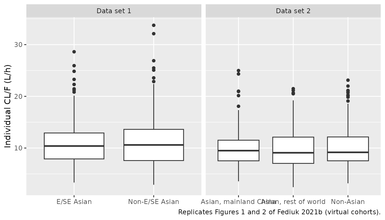
The Results report the median of the post hoc CL/F by group: 10.4 and 10.7 L/h for E/SE Asian and non-E/SE Asian subjects, and 9.42, 9.51 and 10.1 L/h for Asian subjects from mainland China, Asian subjects from the ROW and non-Asian subjects. The lower body weight of the Asian groups offsets most of their higher typical CL/F.
The comparison uses the covariate-driven CL/F of each virtual subject (the random effect removed). Post hoc estimates from the sparsely sampled phase 3 studies shrink towards that value, and the median of 200 drawn random effects adds a few percent of sampling noise that has nothing to do with the covariate model under test; the median including the random effect is shown alongside.
cl_check <- cl_all |>
  group_by(model, group) |>
  summarise(
    model_median = median(cl_typ), model_median_eta = median(cl),
    .groups = "drop"
  ) |>
  left_join(
    tribble(
      ~group,                  ~published_median,
      "E/SE Asian",            10.4,
      "Non-E/SE Asian",        10.7,
      "Asian, mainland China", 9.42,
      "Asian, rest of world",  9.51,
      "Non-Asian",             10.1
    ),
    by = "group"
  ) |>
  mutate(pct_diff = 100 * (model_median / published_median - 1))

cl_check |>
  rename(
    "Model" = model, "Group" = group,
    "Covariate-driven median CL/F (L/h)" = model_median,
    "Median incl. random effect (L/h)" = model_median_eta,
    "Published post hoc median (L/h)" = published_median, "% difference" = pct_diff
  ) |>
knitr::kable(digits = 2, caption = "Median individual CL/F: virtual cohort vs Results.")| Model | Group | Covariate-driven median CL/F (L/h) | Median incl. random effect (L/h) | Published post hoc median (L/h) | % difference |
|---|---|---|---|---|---|
| Data set 1 | E/SE Asian | 10.48 | 10.39 | 10.40 | 0.74 |
| Data set 1 | Non-E/SE Asian | 10.64 | 10.60 | 10.70 | -0.53 |
| Data set 2 | Asian, mainland China | 9.26 | 9.50 | 9.42 | -1.72 |
| Data set 2 | Asian, rest of world | 9.41 | 9.09 | 9.51 | -1.07 |
| Data set 2 | Non-Asian | 9.90 | 9.17 | 10.10 | -2.03 |
# Covariates are drawn in base R from Table 1 summaries, independently of
# each other, while the paper's post hoc values come from the real joint
# covariate distribution, so a few percent of disagreement is expected. A
# mis-transcribed CL/F, eGFR or ethnicity effect moves a group by 8% or more.
stopifnot(
  abs(median(cl_check$pct_diff)) < 3,
  all(abs(cl_check$pct_diff) < 5)
)
PKNCA validation
The paper reports no NCA values, but its AUCtau,ss statements are checkable by NCA. The same 100 virtual subjects (non-Asian demographics of data set 2) receive 15 mg once daily for 14 days under every ethnicity setting of each model, so the per-subject ratio of steady-state AUCtau isolates the ethnicity effect. (Seven days leaves the slowest-clearing subjects of data set 2, whose peripheral volume is larger, about 1.5% short of steady state.) Cmax is reported alongside: the larger Vc/F of the Asian groups lowers Cmax, which the paper notes but does not quantify.
set.seed(20211102)
n_pk <- 100
base_pk <- make_group(n_pk, "base",
  wt = c(89.1, 19.4, 43.4, 197), age = c(55.8, 11.8, 18, 87),
  egfr = c(85.7, 24.6, 6.8, 196), female = 0.440, t2dm = 0.910,
  omega2 = 0.1
) |>
  mutate(subject = row_number()) |>
  select(-group)

arms <- tribble(
  ~model,       ~treatment,                ~RACE_ASIAN, ~REGION_EASTASIA, ~REGION_CHINA,
  "Data set 1", "Non-E/SE Asian",          0,           0,                0,
  "Data set 1", "E/SE Asian",              1,           1,                0,
  "Data set 2", "Non-Asian",               0,           0,                0,
  "Data set 2", "Asian, mainland China",   1,           0,                1,
  "Data set 2", "Asian, rest of world",    1,           0,                0
)

dose_times <- seq(0, 312, by = 24)
obs_times <- sort(unique(c(0, seq(312, 336, by = 0.25))))

make_arm_events <- function(arm) {
  subj <- base_pk |>
    select(-RACE_ASIAN, -REGION_EASTASIA, -REGION_CHINA) |>
    mutate(
      id = subject, treatment = arm$treatment,
      RACE_ASIAN = arm$RACE_ASIAN, REGION_EASTASIA = arm$REGION_EASTASIA,
      REGION_CHINA = arm$REGION_CHINA
    )
  bind_rows(
    subj |> tidyr::crossing(time = dose_times) |>
      mutate(evid = 1L, amt = 15, cmt = "depot"),
    subj |> tidyr::crossing(time = obs_times) |>
      mutate(evid = 0L, amt = 0, cmt = "central")
  ) |>
    arrange(id, time, desc(evid))
}

# One PKNCA call per arm keeps each call small.
nca_arm <- function(i) {
  arm <- arms[i, ]
  mod <- if (arm$model == "Data set 1") mod_esea_typ else mod_china_typ
  ev <- make_arm_events(arm)
  sim <- rxode2::rxSolve(mod, ev, keep = c("treatment", "subject"), returnType = "data.frame")
  conc <- sim |>
    filter(!is.na(Cc), time >= 312) |>
    select(subject, time, Cc, treatment)
  dose <- ev |>
    filter(evid == 1) |>
    select(subject, time, amt, treatment)
  res <- PKNCA::pk.nca(PKNCA::PKNCAdata(
    PKNCA::PKNCAconc(conc, Cc ~ time | treatment + subject),
    PKNCA::PKNCAdose(dose, amt ~ time | treatment + subject),
    intervals = data.frame(start = 312, end = 336, cmax = TRUE, auclast = TRUE)
  ))
  as.data.frame(res$result) |>
    filter(PPTESTCD %in% c("cmax", "auclast")) |>
    mutate(model = arm$model) |>
    left_join(
      sim |> distinct(subject, cl, fdepot),
      by = "subject"
    )
}
nca_all <- bind_rows(lapply(seq_len(nrow(arms)), nca_arm))
#> ℹ omega/sigma items treated as zero: 'etalcl'
#> Warning: multi-subject simulation without without 'omega'
#> ℹ omega/sigma items treated as zero: 'etalcl'
#> Warning: multi-subject simulation without without 'omega'
#> ℹ omega/sigma items treated as zero: 'etalcl'
#> Warning: multi-subject simulation without without 'omega'
#> ℹ omega/sigma items treated as zero: 'etalcl'
#> Warning: multi-subject simulation without without 'omega'
#> ℹ omega/sigma items treated as zero: 'etalcl'
#> Warning: multi-subject simulation without without 'omega'
stopifnot(nrow(nca_all) == 2 * n_pk * nrow(arms))
# Solve against its own closed form: AUCtau at steady state = F * dose / CL.
auc_cf <- nca_all |>
  filter(PPTESTCD == "auclast") |>
  mutate(closed_form = 1000 * 15 * fdepot / cl, pct = 100 * (PPORRES / closed_form - 1))
stopifnot(all(abs(auc_cf$pct) < 1))
reference_arm <- c("Data set 1" = "Non-E/SE Asian", "Data set 2" = "Non-Asian")
nca_ratio <- nca_all |>
  select(model, treatment, subject, PPTESTCD, PPORRES) |>
  group_by(model) |>
  mutate(ref = reference_arm[model]) |>
  ungroup()
nca_ref <- nca_ratio |>
  filter(treatment == ref) |>
  select(model, subject, PPTESTCD, ref_value = PPORRES)
nca_gmr <- nca_ratio |>
  filter(treatment != ref) |>
  left_join(nca_ref, by = c("model", "subject", "PPTESTCD")) |>
  group_by(model, treatment, PPTESTCD) |>
  summarise(gmr = exp(mean(log(PPORRES / ref_value))), .groups = "drop") |>
  pivot_wider(names_from = PPTESTCD, values_from = gmr) |>
  mutate(
    published_auc = c(
      "E/SE Asian" = 0.855, "Asian, mainland China" = 0.962,
      "Asian, rest of world" = 0.917
    )[treatment]
  )

nca_gmr |>
  select(model, treatment, auclast, published_auc, cmax) |>
  rename(
    "Model" = model, "Group vs reference" = treatment,
    "AUCtau,ss GMR (PKNCA)" = auclast, "AUCtau,ss ratio (published)" = published_auc,
    "Cmax,ss GMR (PKNCA)" = cmax
  ) |>
knitr::kable(digits = 3, caption = "Steady-state 15 mg QD exposure ratios vs the reference group.")| Model | Group vs reference | AUCtau,ss GMR (PKNCA) | AUCtau,ss ratio (published) | Cmax,ss GMR (PKNCA) |
|---|---|---|---|---|
| Data set 1 | E/SE Asian | 0.855 | 0.855 | 0.739 |
| Data set 2 | Asian, mainland China | 0.962 | 0.962 | 0.907 |
| Data set 2 | Asian, rest of world | 0.926 | 0.917 | 0.805 |
gmr <- setNames(nca_gmr$auclast, nca_gmr$treatment)
stopifnot(
  abs(gmr[["E/SE Asian"]] - 0.855) < 0.005,
  abs(gmr[["Asian, mainland China"]] - 0.962) < 0.005,
  # 1 / 1.08 = 0.926; the published 0.917 is 1 / 1.09 (bootstrap median).
  abs(gmr[["Asian, rest of world"]] - 1 / 1.08) < 0.005,
  # Larger Vc/F lowers Cmax in every Asian group.
  all(nca_gmr$cmax < 1)
)
The PKNCA AUCtau,ss ratios reproduce the published 0.855 (E/SE Asian) and 0.962 (Asian from mainland China). For Asian subjects from the ROW the model gives 0.926 against the published 0.917; see below.
Assumptions and deviations
-
Ethnicity built from race and region columns. The
paper’s EASIA, RACE2 and RACE3 indicators combine self-reported Asian
ethnicity with the enrollment location, so the models build them as
products of
RACE_ASIANwithREGION_EASTASIA/REGION_SOUTHEASTASIA(data set 1) orREGION_CHINA(data set 2). The paper also counts every Japanese subject of the Japanese/Western phase 1 PK/PD study as E/SE Asian; code those subjectsRACE_ASIAN = 1, REGION_EASTASIA = 1. Hong Kong and Taiwan sites are East Asian in data set 1 and “rest of the world” in data set 2 (mainland China only). - ROW Asian AUCtau,ss ratio. The Results give 0.917 (95% CI 0.877-0.971) for Asian subjects from the ROW. The Table 2 point estimate 1.08 gives 1 / 1.08 = 0.926; the published value equals 1 / 1.09, the bootstrap median in the same Table 2 row, as the 95% CI equals 1 / (1.14, 1.03). The packaged model uses the point estimate 1.08, like every other parameter.
-
Food effects on ka and F1 follow the parent
analysis parameterization (multiplicative on ka;
F1 = 1 - theta_fed * FED - theta_missing * FED_MISSING), which Fediuk 2021b states it inherits; Table S3 prints only the CL/F, Vc/F, Vp/F and Q/F equations. “Without regard to food” (the phase 3 setting) is theFED_MISSINGlevel. -
Residual error is on the SD scale, as in the parent
analysis: the Results report the residual errors as 38.9%/83.7% (data
set 1) and 48.6%/83.1% (data set 2), the Table 2 values times 100, while
the omega^2 rows are variances (31.8% = sqrt(0.101)). The phase 2 and
phase 3 studies share one SD, selected by
STUDY_PHASE2orSTUDY_PHASE3. -
eGFR cap. The authors set eGFR above 120
mL/min/1.73 m^2 to 120;
model()applies the same cap. - Virtual cohorts draw body weight, age and eGFR independently from the Table 1 group summaries; correlations between them are not reproduced. All cohorts are dosed fasted with the phase 1 residual stratum.
- No erratum was found for this article (Europe PMC search, 2026-10-02).