Erenumab immune tolerance in rats (Gupta 2025)
Source:vignettes/articles/Gupta_2025_erenumab_rat.Rmd
Gupta_2025_erenumab_rat.RmdModel and source
- Citation: Gupta P, Ryman JT, Jawa V, Meibohm B. A Semi-Mechanistic Mathematical Model of Immune Tolerance Induction to Support Preclinical Studies of Human Monoclonal Antibodies in Rats. Pharmaceutics. 2025;17(7):845. doi:10.3390/pharmaceutics17070845. PK parameters from Table 1; immune-cell parameters from Table 2 and Supplementary Table S1; equations from Equations 1-12 and Supplementary Equations S1-S15.
- Description: Preclinical (rat). QSP. Integrated PK / semi-mechanistic immune-cell model of anti-drug antibody (ADA) formation and immune tolerance induction against the human IgG2 monoclonal antibody erenumab in Sprague-Dawley rats (Gupta 2025): one-compartment first-order absorption erenumab PK with aggregation-state effects on CL/F and ka and an ADA-magnitude power effect on CL/F, driving dendritic-cell maturation and CD4+ T-helper / T-regulatory cell activation and proliferation; tacrolimus (inhibits T-helper proliferation) and methotrexate (inhibits T-helper activation) carried as coupled one-compartment PK states.
- Article: https://doi.org/10.3390/pharmaceutics17070845 (open access; the supplement with Equations S1-S15 and Table S1 is at https://www.mdpi.com/article/10.3390/pharmaceutics17070845/s1)
Gupta 2025 built the model in two steps. A one-compartment population PK model of erenumab in rats (Monolix, Table 1) used the observed ADA signal-to-noise ratio (S/N) as a time-varying covariate on clearance. The individual PK profiles then drove a semi-mechanistic model of dendritic cells, CD4+ T-helper cells and T-regulatory cells, whose activated T-helper count generates the ADA response (Table 2, Figure 2). Methotrexate inhibits the activation of naive T-helper cells and tacrolimus inhibits the proliferation of activated T-helper cells.
The packaged model joins the two steps the way Figure 2 draws them:
the model-predicted ADA S/N, rather than an observed S/N column, enters
the clearance term of Equation 4, so ADA formation feeds back on
erenumab exposure. Tacrolimus and methotrexate are carried as their own
one-compartment PK states (doses in mg/kg into
depot_tacrolimus and depot_methotrexate),
which reproduces the multiple-dose concentration Equations S12 and S14
for any regimen.
Population
Two 12-week immune-tolerance studies in Sprague-Dawley rats (Gupta 2025 Section 2.1, Figure 1), each split into an induction phase (weeks 1-4), a washout phase (weeks 5-8) and a rechallenge phase (weeks 9-12). Erenumab was given SC once weekly in weeks 1-4 and 9-12: 10 mg/kg monomer in Study 1 and 1 mg/kg aggregates in Study 2. Study 1 had four groups of 8 animals (1.1 control; 1.2 methotrexate 5 mg/kg IP weekly in weeks 1-7; 1.3 methotrexate 3 mg/kg IP on days 1-3; 1.4 sirolimus 6 mg/kg PO on day 1 plus tacrolimus 2 mg/kg SC weekly in weeks 1-7), and Study 2 had two groups of 10 (2.1 control; 2.2 tacrolimus/sirolimus as in 1.4). The analysis used 1924 erenumab concentrations and 624 ADA measurements from 52 animals, 14 of them ADA-positive. Animals weighed about 270-290 g at purchase and 380-410 g at week 12 (Discussion). Sex was not reported.
The same information is available programmatically via
readModelDb("Gupta_2025_erenumab_rat")()$population.
Source trace
| Equation / parameter | Value | Source location |
|---|---|---|
lka (ka, monomer) |
0.91 1/day | Table 1 |
lcl (CL/F, monomer, ADA-negative) |
1.83 mL/day | Table 1 |
lvc (Vd/F) |
32.6 mL | Table 1 |
e_aggregate_cl |
2.40 | Table 1, Equation 3 |
e_aggregate_ka |
0.12 | Table 1, Equation 3 |
e_ada_cl |
0.37 | Table 1, Equation 4 |
sn_cutoff, sn_cutoff_s2
|
2, 1.5 | Section 2.1 (ADA-positivity threshold); Figure 2 legend |
etalcl |
0.178^2 | Table 1 (IIV 17.8%) |
etalvc, etalvc_s2
|
0.869^2, 0.212^2 | Table 1 (IIV 86.9% Study 1, 21.2% Study 2) |
etaiov_lka_1 … _8
|
1.83^2 | Table 1 (IOV 183%), Section 2.2.1 (eight occasions) |
addSd, propSd
|
0.09 ug/mL, 0.29 | Table 1 (Study 1) |
addSd_s2, propSd_s2
|
0.12 ug/mL, 0.13 | Table 1 (Study 2) |
betaND, ND0, deltaND
|
0.0924 1/day, 3700 cells/uL, 1.5 1/day | Table 2 C, Table S1 |
ec50, ec50_aggregate
|
9.85, 2.02 ug/mL | Table 2 C and A |
betaMD |
0.2310 1/day | Table 2 C |
NThlp0, betaNThlp,
deltaNThlp
|
723 cells/uL, 0.0056 1/day, 1.5 1/day | Table 2 C |
rhoAThlp, betaAThlp
|
2.45 1/day, 0.05 1/day | Table 2 A |
NTreg0, betaNTreg,
deltaNTreg
|
62 cells/uL, 0.0056 1/day, 1.5 1/day | Table 2 C |
betaATreg |
0.18 1/day | Table 2 C |
lrhoATreg, etalrhoATreg
|
3.02 1/day, 0.153^2 | Table 2 B |
lATreg50, etalATreg50
|
1000 cells/uL, 0.034^2 | Table 2 B |
ltlag_ada, etaltlag_ada
|
28.3 day, 0.53^2 | Table 2 B |
alphaADA, kADA
|
77 nmol/day, 0.138 1/day | Table 2 C |
kADAprop (K), nADA (N) |
500 cells/day, 1000 nmol/uL | Table S1 |
Tacrolimus f_, ka_, kel_,
vc_, ic50_tacrolimus
|
0.2, 7.2 1/day, 3.6 1/day, 10 L/kg, 0.2 nM | Table S1; Section 2.2.2 |
Methotrexate f_, ka_, kel_,
vc_, ic50_methotrexate
|
1, 88.56 1/day, 56.41 1/day, 0.174 L/kg, 1 nM | Table S1; Section 2.2.2 |
mw_tacrolimus, mw_methotrexate
|
804.02, 454.44 g/mol | Molecular formulae (not in the source) |
d/dt(depot), d/dt(central)
|
n/a | Equations 5, S1-S2 |
d/dt(ND), d/dt(MD)
|
n/a | Equations 6, S4-S5 |
d/dt(NThlp), d/dt(AThlp)
|
n/a | Equations 7, 11, 12, S6, S7, S13, S15 |
d/dt(NTreg), d/dt(ATreg)
|
n/a | Equations 8, S8-S9 |
D |
n/a | Equation 9 |
ada, ada_sn
|
n/a | Equations 10, S10-S11 |
| ADA effect on CL/F | n/a | Equation 4 |
| Tacrolimus / methotrexate concentrations | n/a | Equations S12, S14 |
Virtual cohort
The six treatment groups of Figure 1 are rebuilt with 100 virtual animals each. Erenumab doses are mg/kg, so the absolute amount needs a body weight. The paper does not report individual weights. Body weight is taken to rise linearly from 0.28 kg on day 0 to 0.395 kg on day 84, the midpoints of the ranges given in the Discussion.
set.seed(2025)

ere_days <- c(0, 7, 14, 21, 56, 63, 70, 77)
obs_days <- sort(unique(c(seq(0, 84, by = 0.5), 0.1, 0.3)))
wt_kg <- function(t) 0.28 + (0.395 - 0.28) * t / 84

groups <- tibble::tribble(
  ~group,                        ~study2, ~agg, ~ere_mgkg, ~imm,
  "1.1 Control (monomer)",       0,       0,    10,        "none",
  "1.2 MTX 5 mg/kg weekly",      0,       0,    10,        "mtx5",
  "1.3 MTX 3 mg/kg days 1-3",    0,       0,    10,        "mtx3",
  "1.4 TAC/SIR (monomer)",       0,       0,    10,        "tac",
  "2.1 Control (aggregates)",    1,       1,    1,         "none",
  "2.2 TAC/SIR (aggregates)",    1,       1,    1,         "tac"
)

make_group <- function(g, n, id_offset, obs = obs_days, ere = ere_days) {
  doses <- tibble(time = ere, evid = 1L, cmt = "depot",
                  amt = g$ere_mgkg * wt_kg(ere) * 1000)
  imm <- switch(
    g$imm,
    none = NULL,
    mtx5 = tibble(time = seq(0, 42, by = 7), evid = 1L, cmt = "depot_methotrexate", amt = 5),
    mtx3 = tibble(time = 0:2, evid = 1L, cmt = "depot_methotrexate", amt = 3),
    tac  = tibble(time = seq(0, 42, by = 7), evid = 1L, cmt = "depot_tacrolimus", amt = 2)
  )
  obs_rows <- tibble(time = obs, evid = 0L, cmt = "central", amt = 0)
  one <- bind_rows(doses, imm, obs_rows) |>
    arrange(time, desc(evid))
  # One ka occasion per erenumab dose: OCC = number of erenumab doses so far.
  one$OCC <- pmax(1L, findInterval(one$time, ere))
  tidyr::crossing(id = id_offset + seq_len(n), one) |>
    mutate(
      group = g$group,
      FORM_ERENUMAB_AGGREGATE = g$agg,
      STUDY_ERENUMAB_S2 = g$study2
    ) |>
    arrange(id, time, desc(evid))
}

n_per_group <- 100
events <- bind_rows(lapply(seq_len(nrow(groups)), function(i) {
  make_group(groups[i, ], n_per_group, id_offset = (i - 1L) * n_per_group)
}))
stopifnot(!anyDuplicated(events[, c("id", "time", "evid", "cmt")]))
Simulation
mod <- readModelDb("Gupta_2025_erenumab_rat")
keep_cols <- c("group", "FORM_ERENUMAB_AGGREGATE", "STUDY_ERENUMAB_S2")

rxode2::rxSetSeed(2025)
sim <- rxode2::rxSolve(mod, events = events, keep = keep_cols) |>
  as.data.frame()
#> ℹ parameter labels from comments will be replaced by 'label()'
#> Warning: some etas defaulted to non-mu referenced, possible parsing error: etalvc, etalvc_s2, etaiov_lka_1, etaiov_lka_2, etaiov_lka_3, etaiov_lka_4, etaiov_lka_5, etaiov_lka_6, etaiov_lka_7, etaiov_lka_8
#> as a work-around try putting the mu-referenced expression on a simple line

# Typical-value animal per group (all random effects zero).
mod_typ <- rxode2::zeroRe(mod)
#> ℹ parameter labels from comments will be replaced by 'label()'
#> Warning: some etas defaulted to non-mu referenced, possible parsing error: etalvc, etalvc_s2, etaiov_lka_1, etaiov_lka_2, etaiov_lka_3, etaiov_lka_4, etaiov_lka_5, etaiov_lka_6, etaiov_lka_7, etaiov_lka_8
#> as a work-around try putting the mu-referenced expression on a simple line
#> Warning: No sigma parameters in the model
#> Warning: some etas defaulted to non-mu referenced, possible parsing error: etalvc, etalvc_s2, etaiov_lka_1, etaiov_lka_2, etaiov_lka_3, etaiov_lka_4, etaiov_lka_5, etaiov_lka_6, etaiov_lka_7, etaiov_lka_8
#> as a work-around try putting the mu-referenced expression on a simple line
events_typ <- bind_rows(lapply(seq_len(nrow(groups)), function(i) {
  make_group(groups[i, ], 1, id_offset = i - 1L)
}))
sim_typ <- rxode2::rxSolve(mod_typ, events = events_typ, keep = keep_cols) |>
  as.data.frame()
#> ℹ omega/sigma items treated as zero: 'etalcl', 'etalvc', 'etalvc_s2', 'etaiov_lka_1', 'etaiov_lka_2', 'etaiov_lka_3', 'etaiov_lka_4', 'etaiov_lka_5', 'etaiov_lka_6', 'etaiov_lka_7', 'etaiov_lka_8', 'etalrhoATreg', 'etalATreg50', 'etaltlag_ada'
#> Warning: multi-subject simulation without without 'omega'
Erenumab pharmacokinetics
Closed-form check of the PK layer
While the typical animal stays below the ADA-positivity cut-off, CL/F is constant and Equation 5 has the closed-form multiple-dose solution below. The solved profile of the typical control animal (Group 1.1) is checked against it. Both sides use the same parameters, so the difference is integration error only.
typ_ctl <- sim_typ |> filter(group == "1.1 Control (monomer)")
stopifnot(max(typ_ctl$ada_sn) < 2)

ka <- 0.91; cl <- 1.83; vc <- 32.6; k <- cl / vc
dose_amt <- 10 * wt_kg(ere_days) * 1000
closed <- vapply(typ_ctl$time, function(t) {
  sum(ifelse(t >= ere_days,
             dose_amt * ka / (vc * (ka - k)) *
               (exp(-k * (t - ere_days)) - exp(-ka * (t - ere_days))), 0))
}, numeric(1))
rel_err <- abs(typ_ctl$Cc - closed)[closed > 1] / closed[closed > 1]
max(rel_err)
#> [1] 7.053784e-07
stopifnot(max(rel_err) < 1e-3)
Concentration-time profiles
# Compare with Figures 3 and 5 of Gupta 2025: erenumab serum concentrations by
# treatment group (observed data and VPC in the paper).
sim |>
  filter(time != 0) |>
  group_by(group, time) |>
  summarise(
    Q05 = quantile(Cc, 0.05),
    Q50 = quantile(Cc, 0.50),
    Q95 = quantile(Cc, 0.95),
    .groups = "drop"
  ) |>
  ggplot(aes(time, Q50)) +
  geom_ribbon(aes(ymin = Q05, ymax = Q95), alpha = 0.25, fill = "steelblue") +
  geom_line(colour = "steelblue4") +
  facet_wrap(~group, ncol = 2) +
  scale_y_log10() +
  scale_x_continuous(breaks = seq(0, 84, 14)) +
  labs(x = "Time (day)", y = "Erenumab (ug/mL)",
       title = "Simulated median and 90% interval, 100 animals per group",
       caption = "Compare with Figures 3 and 5 of Gupta 2025.")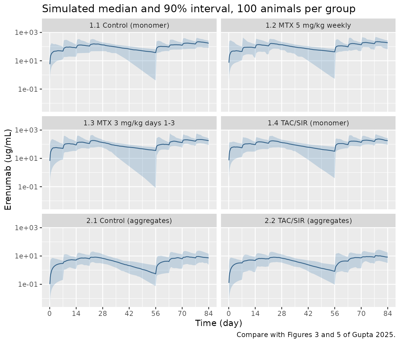
The aggregate groups have lower and later peaks than the monomer groups because of the 10-fold lower dose, the 2.4-fold higher CL/F and the 8-fold slower absorption (Table 1). The wide intervals in Study 1 come from the 86.9% IIV on Vd/F and the very large inter-occasion variability on ka.
PKNCA
Gupta 2025 reports no NCA, so the table below characterises the simulated first dosing interval (days 0-7) and the last rechallenge interval (days 77-84) without a published comparator.
sim_nca <- sim |>
  filter(!is.na(Cc)) |>
  select(id, time, Cc, group)
sim_nca <- bind_rows(
  sim_nca,
  sim_nca |> distinct(id, group) |> mutate(time = 0, Cc = 0)
) |>
  distinct(id, group, time, .keep_all = TRUE) |>
  arrange(id, group, time)

dose_df <- events |>
  filter(evid == 1, cmt == "depot") |>
  select(id, time, amt, group)

conc_obj <- PKNCA::PKNCAconc(sim_nca, Cc ~ time | group + id)
dose_obj <- PKNCA::PKNCAdose(dose_df, amt ~ time | group + id)
intervals <- data.frame(
  start = c(0, 77), end = c(7, 84),
  cmax = TRUE, tmax = TRUE, auclast = TRUE
)
nca_res <- PKNCA::pk.nca(PKNCA::PKNCAdata(conc_obj, dose_obj, intervals = intervals))

as.data.frame(nca_res) |>
  filter(PPTESTCD %in% c("cmax", "tmax", "auclast")) |>
  group_by(group, start, end, PPTESTCD) |>
  summarise(median = signif(median(PPORRES, na.rm = TRUE), 3), .groups = "drop") |>
  tidyr::pivot_wider(names_from = PPTESTCD, values_from = median) |>
  mutate(interval = paste0(start, "-", end, " d")) |>
  select(group, interval, cmax, tmax, auclast) |>
  rename(
    "Group" = group,
    "Interval" = interval,
    "Cmax (ug/mL)" = cmax,
    "Tmax (day)" = tmax,
    "AUC (ug*day/mL)" = auclast
  ) |>
knitr::kable(caption = "Median simulated NCA parameters by group and dosing interval.")| Group | Interval | Cmax (ug/mL) | Tmax (day) | AUC (ug*day/mL) |
|---|---|---|---|---|
| 1.1 Control (monomer) | 0-7 d | 52.90 | 3.5 | 298.0 |
| 1.1 Control (monomer) | 77-84 d | 228.00 | 2.0 | 1400.0 |
| 1.2 MTX 5 mg/kg weekly | 0-7 d | 52.10 | 3.0 | 324.0 |
| 1.2 MTX 5 mg/kg weekly | 77-84 d | 228.00 | 1.5 | 1440.0 |
| 1.3 MTX 3 mg/kg days 1-3 | 0-7 d | 62.40 | 3.5 | 370.0 |
| 1.3 MTX 3 mg/kg days 1-3 | 77-84 d | 221.00 | 1.5 | 1440.0 |
| 1.4 TAC/SIR (monomer) | 0-7 d | 69.70 | 3.5 | 412.0 |
| 1.4 TAC/SIR (monomer) | 77-84 d | 239.00 | 1.5 | 1490.0 |
| 2.1 Control (aggregates) | 0-7 d | 3.03 | 7.0 | 14.6 |
| 2.1 Control (aggregates) | 77-84 d | 10.60 | 2.0 | 57.5 |
| 2.2 TAC/SIR (aggregates) | 0-7 d | 3.32 | 7.0 | 16.7 |
| 2.2 TAC/SIR (aggregates) | 77-84 d | 12.00 | 1.5 | 68.7 |
Immune-cell kinetics and ADA
Typical-value animal in each group
# Compare with the ADA-negative panels of Figures 6-9 of Gupta 2025.
sim_typ |>
  select(group, time, AThlp, ATreg) |>
  pivot_longer(c(AThlp, ATreg), names_to = "cell", values_to = "count") |>
  ggplot(aes(time, count, colour = cell)) +
  geom_line() +
  facet_wrap(~group, ncol = 2) +
  scale_colour_manual(values = c(AThlp = "forestgreen", ATreg = "darkorange")) +
  scale_x_continuous(breaks = seq(0, 84, 14)) +
  labs(x = "Time (day)", y = "Cells/uL", colour = NULL,
       title = "Activated T-helper and T-regulatory cells, typical animal",
       caption = "Compare with the ADA-negative panels of Figures 6-9 of Gupta 2025.")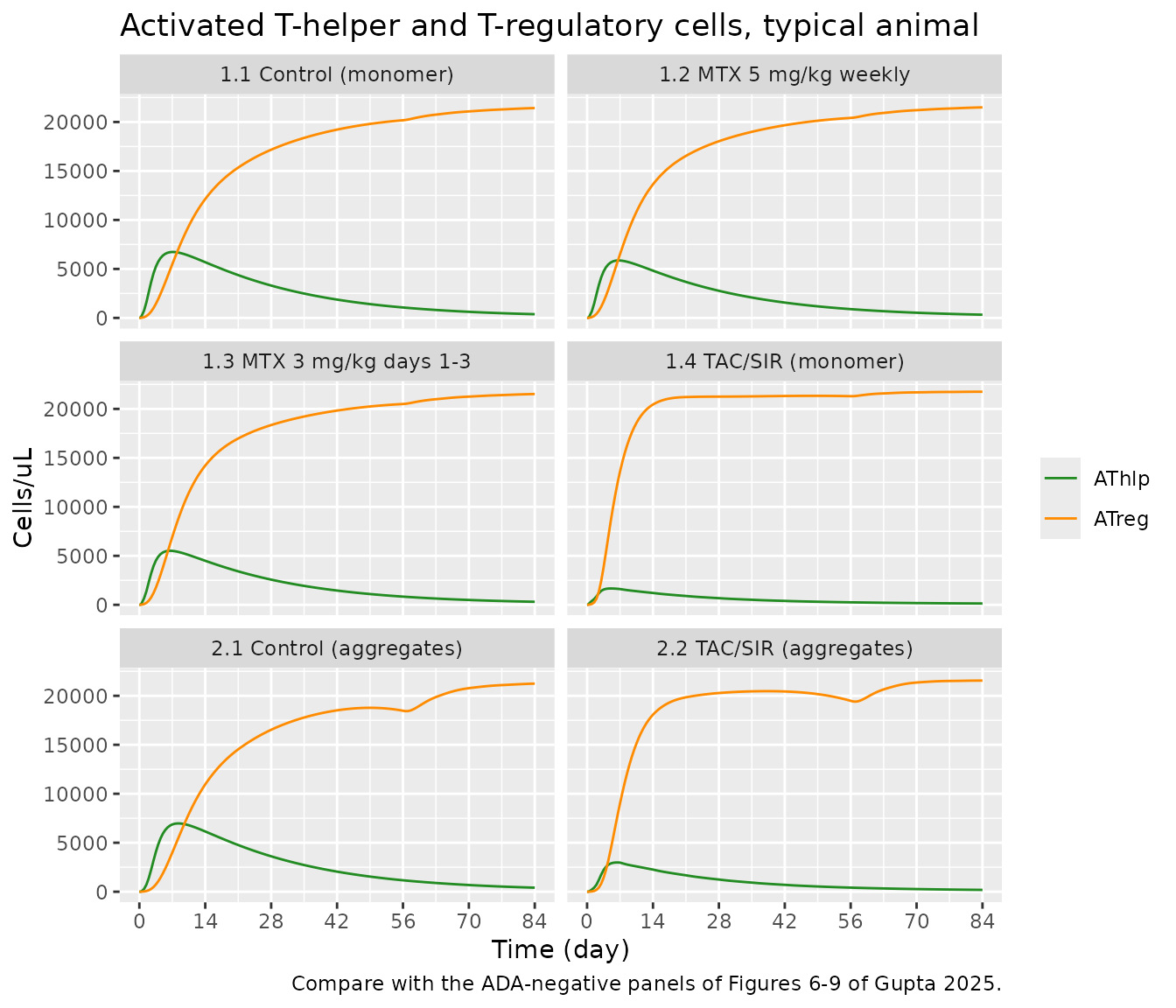
typ_sum <- sim_typ |>
  group_by(group) |>
  summarise(
    AThlp_d28 = AThlp[time == 28],
    ATreg_d28 = ATreg[time == 28],
    AThlp_d84 = AThlp[time == 84],
    ATreg_d84 = ATreg[time == 84],
    max_sn = max(ada_sn),
    .groups = "drop"
  )
typ_sum |>
  mutate(across(where(is.numeric), \(x) signif(x, 3))) |>
  rename(
    "Group" = group,
    "AThlp day 28" = AThlp_d28,
    "ATreg day 28" = ATreg_d28,
    "AThlp day 84" = AThlp_d84,
    "ATreg day 84" = ATreg_d84,
    "Max ADA S/N" = max_sn
  ) |>
knitr::kable(caption = "Typical-value cell counts (cells/uL) at the end of induction and rechallenge.")| Group | AThlp day 28 | ATreg day 28 | AThlp day 84 | ATreg day 84 | Max ADA S/N |
|---|---|---|---|---|---|
| 1.1 Control (monomer) | 3300 | 17200 | 379 | 21400 | 0.2510 |
| 1.2 MTX 5 mg/kg weekly | 2770 | 18000 | 328 | 21500 | 0.2100 |
| 1.3 MTX 3 mg/kg days 1-3 | 2570 | 18400 | 310 | 21500 | 0.1950 |
| 1.4 TAC/SIR (monomer) | 679 | 21300 | 137 | 21800 | 0.0528 |
| 2.1 Control (aggregates) | 3620 | 16500 | 412 | 21200 | 0.2750 |
| 2.2 TAC/SIR (aggregates) | 1250 | 20300 | 187 | 21600 | 0.0937 |
# The typical animal stays ADA-negative in every group, as most animals did
# (36 of 52 ADA-negative; Section 3).
cut_by_group <- ifelse(grepl("^2", typ_sum$group), 1.5, 2)
stopifnot(all(typ_sum$max_sn < cut_by_group))
# Tacrolimus inhibits T-helper proliferation: fewer activated T-helper cells
# than in the matching control at the end of induction.
stopifnot(
  typ_sum$AThlp_d28[typ_sum$group == "1.4 TAC/SIR (monomer)"] <
    typ_sum$AThlp_d28[typ_sum$group == "1.1 Control (monomer)"],
  typ_sum$AThlp_d28[typ_sum$group == "2.2 TAC/SIR (aggregates)"] <
    typ_sum$AThlp_d28[typ_sum$group == "2.1 Control (aggregates)"]
)
In the ADA-negative animals of Figures 6b, 7 and 8b the activated T-regulatory cells reach roughly 20,000-55,000 cells/uL and outnumber the activated T-helper cells, which return towards zero. The typical-value animals above behave the same way, with T-regulatory counts of about 21,000 cells/uL at the lower end of that range.
An ADA-positive animal
ADA formation in this model hinges on the T-regulatory proliferation
rate rhoATreg, the most sensitive parameter in the paper’s
sensitivity analysis (Table 3, CCmax -85). An animal at the 2.5th
percentile of its distribution,
rhoATreg = 3.02 * exp(-1.96 * 0.153), is simulated without
immunosuppression.
# Compare with Figure 6a of Gupta 2025 (Group 1.1, ADA-positive animals).
rho_low <- 3.02 * exp(-1.96 * 0.153)
sim_pos <- rxode2::rxSolve(
  mod_typ,
  events = events_typ |> filter(group == "1.1 Control (monomer)"),
  params = c(lrhoATreg = log(rho_low))
) |>
  as.data.frame()
#> ℹ omega/sigma items treated as zero: 'etalcl', 'etalvc', 'etalvc_s2', 'etaiov_lka_1', 'etaiov_lka_2', 'etaiov_lka_3', 'etaiov_lka_4', 'etaiov_lka_5', 'etaiov_lka_6', 'etaiov_lka_7', 'etaiov_lka_8', 'etalrhoATreg', 'etalATreg50', 'etaltlag_ada'

p_cells <- sim_pos |>
  select(time, AThlp, ATreg) |>
  pivot_longer(-time, names_to = "cell", values_to = "count") |>
  ggplot(aes(time, count, colour = cell)) +
  geom_line() +
  scale_colour_manual(values = c(AThlp = "forestgreen", ATreg = "darkorange")) +
  labs(x = "Time (day)", y = "Cells/uL", colour = NULL)
p_ada <- ggplot(sim_pos, aes(time, pmax(ada_sn, 1e-3))) +
  geom_line(colour = "blue") +
  geom_hline(yintercept = 2, linetype = "dashed") +
  scale_y_log10() +
  labs(x = "Time (day)", y = "ADA S/N")
p_cells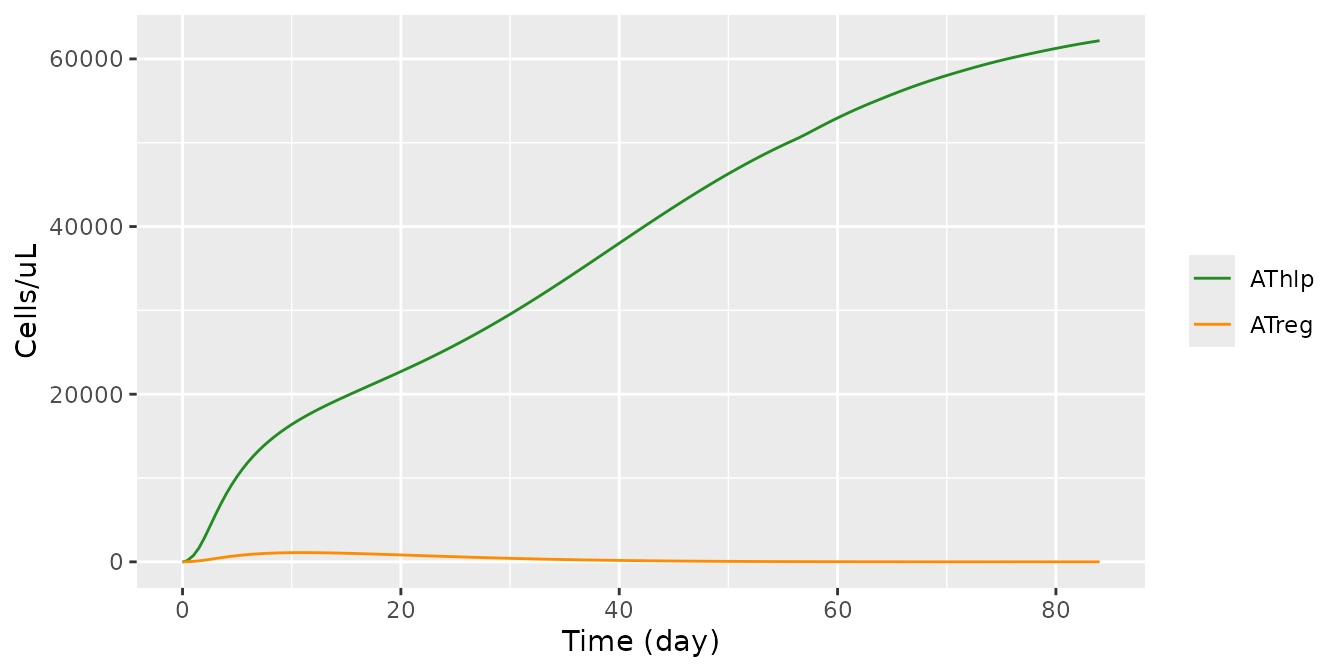
p_ada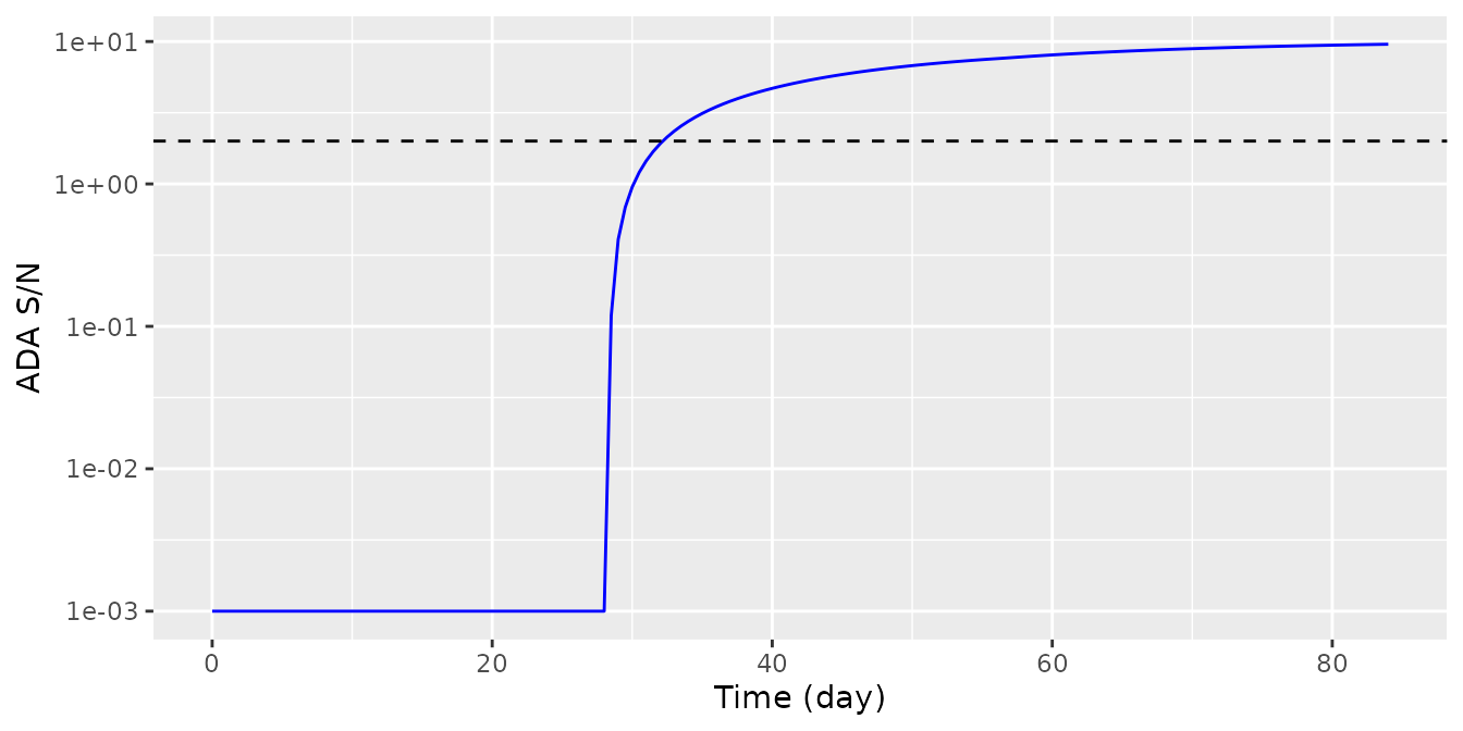
stopifnot(
  sim_pos$AThlp[sim_pos$time == 35] > sim_pos$ATreg[sim_pos$time == 35],
  max(sim_pos$ada_sn) > 2
)
The ADA-positive branch has activated T-helper cells outnumbering activated T-regulatory cells, as in Figure 6a, and the predicted S/N crosses the cut-off after the 28-day lag. Its magnitude, however, stays within about one log unit of the cut-off, whereas the predicted curves in Figure 6a climb to S/N 104-105 (see Assumptions and deviations).
ADA incidence by group
Each virtual animal is classified ADA-positive when its predicted S/N exceeds the study’s cut-off at any time during the 12 weeks.
observed_incidence <- tibble::tribble(
  ~group,                       ~observed,
  "1.1 Control (monomer)",      "2/8 (25%)",
  "1.2 MTX 5 mg/kg weekly",     "5/8 (62.5%)",
  "1.3 MTX 3 mg/kg days 1-3",   "1/8 (12.5%)",
  "1.4 TAC/SIR (monomer)",      "0/8 (0%)",
  "2.1 Control (aggregates)",   "6/10 (60%)",
  "2.2 TAC/SIR (aggregates)",   "0/10 (0%)"
)
incidence <- sim |>
  mutate(cut = ifelse(STUDY_ERENUMAB_S2 == 1, 1.5, 2)) |>
  group_by(group, id) |>
  summarise(pos = any(ada_sn > cut), .groups = "drop") |>
  group_by(group) |>
  summarise(simulated = mean(pos), .groups = "drop") |>
  left_join(observed_incidence, by = "group")
incidence |>
  mutate(simulated = sprintf("%.0f%%", 100 * simulated)) |>
  rename("Group" = group, "Simulated" = simulated,
         "Observed (Figure 4, Discussion)" = observed) |>
knitr::kable(caption = "ADA incidence: 100 virtual animals per group versus the observed studies.")| Group | Simulated | Observed (Figure 4, Discussion) |
|---|---|---|
| 1.1 Control (monomer) | 7% | 2/8 (25%) |
| 1.2 MTX 5 mg/kg weekly | 6% | 5/8 (62.5%) |
| 1.3 MTX 3 mg/kg days 1-3 | 5% | 1/8 (12.5%) |
| 1.4 TAC/SIR (monomer) | 0% | 0/8 (0%) |
| 2.1 Control (aggregates) | 13% | 6/10 (60%) |
| 2.2 TAC/SIR (aggregates) | 2% | 0/10 (0%) |
The tacrolimus/sirolimus groups are essentially ADA-free, in line
with the studies. The simulated incidence in the control and
methotrexate groups is well below the observed incidence, and the model
does not separate the two methotrexate regimens from their control.
Gupta 2025 fitted the immune model to each animal with its own PK and
its own rhoATreg, ATreg50 and
Tlag, and reports group incidences from those individual
fits, not from a population simulation; a population simulation from the
reported variances is therefore not expected to reproduce them
exactly.
Chronic toxicology study after tolerance induction
Gupta 2025 Section 3.3 simulated a 6-month study in 1000 animals
tolerised with the tacrolimus/sirolimus regimen: weekly 10 mg/kg monomer
in weeks 1-4, tacrolimus in weeks 1-7, then weekly erenumab for 6 months
of rechallenge without immunosuppression. Only rhoATreg was
sampled. Here 200 animals are simulated the same way, with all other
random effects at zero, and erenumab given weekly from week 9 to week
34.
chronic_ere <- c(seq(0, 21, by = 7), seq(56, 231, by = 7))
chronic_obs <- seq(0, 364, by = 1)
n_chronic <- 200
ev_chronic <- make_group(groups[4, ], n_chronic, id_offset = 0L,
                         obs = chronic_obs, ere = chronic_ere) |>
  mutate(
    amt = ifelse(cmt == "depot", 10 * wt_kg(pmin(time, 84)) * 1000, amt),
    OCC = 1L
  )
par_chronic <- data.frame(
  id = seq_len(n_chronic),
  lrhoATreg = log(3.02) + rnorm(n_chronic, 0, 0.153)
)
sim_chronic <- rxode2::rxSolve(mod_typ, events = ev_chronic, params = par_chronic) |>
  as.data.frame()
#> ℹ omega/sigma items treated as zero: 'etalcl', 'etalvc', 'etalvc_s2', 'etaiov_lka_1', 'etaiov_lka_2', 'etaiov_lka_3', 'etaiov_lka_4', 'etaiov_lka_5', 'etaiov_lka_6', 'etaiov_lka_7', 'etaiov_lka_8', 'etalrhoATreg', 'etalATreg50', 'etaltlag_ada'
#> Warning: multi-subject simulation without without 'omega'

chronic_sum <- sim_chronic |>
  select(id, time, AThlp, ATreg, ada_sn) |>
  pivot_longer(c(AThlp, ATreg, ada_sn), names_to = "var", values_to = "value") |>
  group_by(var, time) |>
  summarise(
    mean = mean(value),
    lo = quantile(value, 0.025),
    hi = quantile(value, 0.975),
    .groups = "drop"
  )
ggplot(chronic_sum, aes(time / 7, mean)) +
  geom_ribbon(aes(ymin = lo, ymax = hi), alpha = 0.25) +
  geom_line() +
  facet_wrap(~var, scales = "free_y", ncol = 1,
             labeller = as_labeller(c(AThlp = "Activated T-helper cells (cells/uL)",
                                      ATreg = "Activated T-regulatory cells (cells/uL)",
                                      ada_sn = "ADA S/N"))) +
  labs(x = "Time (week)", y = NULL,
       title = "Mean and 95% interval, 200 tolerised animals",
       caption = "Compare with Figure 10 of Gupta 2025.")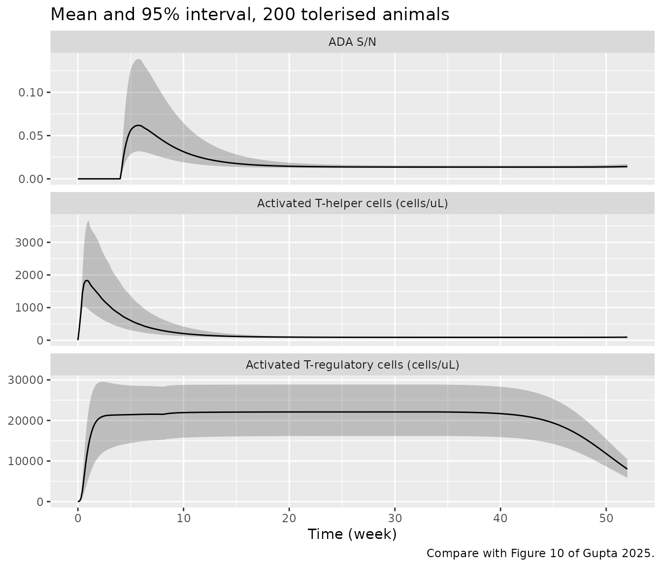
max_sn_chronic <- sim_chronic |> group_by(id) |> summarise(m = max(ada_sn))
fig10 <- tibble::tribble(
  ~quantity,                                   ~published,
  "Peak mean AThlp (cells/uL)",                "about 120, near week 1",
  "Mean ATreg, week 5 (cells/uL)",             "about 30,000",
  "Mean ATreg, weeks 20-34 (cells/uL)",        "about 66,000",
  "Animals ADA-positive (S/N > 2)",            "none",
  "Mean ADA S/N at week 52",                   "about 0.8"
)
mean_at <- function(v, wk) {
  mean(sim_chronic[[v]][sim_chronic$time %in% (wk * 7)])
}
fig10$simulated <- c(
  sprintf("%.0f, week %.1f",
          max(chronic_sum$mean[chronic_sum$var == "AThlp"]),
          chronic_sum$time[chronic_sum$var == "AThlp"][
            which.max(chronic_sum$mean[chronic_sum$var == "AThlp"])] / 7),
  sprintf("%.0f", mean_at("ATreg", 5)),
  sprintf("%.0f", mean_at("ATreg", 20:34)),
  sprintf("%d of %d", sum(max_sn_chronic$m > 2), n_chronic),
  sprintf("%.2f", mean_at("ada_sn", 52))
)
fig10 |>
  rename("Quantity" = quantity, "Figure 10 (read from the plot)" = published,
         "This implementation" = simulated) |>
knitr::kable(caption = "Chronic-study simulation against Figure 10 of Gupta 2025.")| Quantity | Figure 10 (read from the plot) | This implementation |
|---|---|---|
| Peak mean AThlp (cells/uL) | about 120, near week 1 | 1831, week 0.9 |
| Mean ATreg, week 5 (cells/uL) | about 30,000 | 21432 |
| Mean ATreg, weeks 20-34 (cells/uL) | about 66,000 | 22094 |
| Animals ADA-positive (S/N > 2) | none | 0 of 200 |
| Mean ADA S/N at week 52 | about 0.8 | 0.01 |
# Tolerance is maintained: no animal crosses the ADA cut-off.
stopifnot(mean(max_sn_chronic$m > 2) < 0.05)
The qualitative result of Section 3.3 holds: once tolerised, continued erenumab dosing keeps activated T-regulatory cells far above activated T-helper cells and no animal becomes ADA-positive. The magnitudes do not match Figure 10. The early T-helper peak is about 15-fold higher, the T-regulatory plateau during continued dosing is about one third of the published one and does not rise between week 5 and week 20, and the predicted S/N falls with the T-helper count instead of settling at about 0.8. The paper’s own T-cell curves for the same regimen in the 12-week study (Figure 7c, Figure 9) show T-regulatory counts of 20,000-60,000 cells/uL, closer to this implementation; the source does not say what else differed in the Figure 10 simulation.
Assumptions and deviations
-
ADA magnitude does not reproduce the published
curves. Equations 10 and S10-S11 make ADA proportional to the
current activated T-helper count, zero before
Tlag, and the S/N is ADA divided byN. Implemented as printed, an animal with about 10,000 activated T-helper cells has an S/N of about 1.5. The predicted curves in Figures 6-9, though, reach S/N 104-105 at similar T-helper counts, are non-zero beforeTlag, and in Figure 10 the S/N stays at about 0.8 for 40 weeks after the activated T-helper cells have gone. The printed equations cannot produce these curves, and the source gives no other form. The equations are implemented as printed. The qualitative behaviour that carries the paper’s conclusions is reproduced: tacrolimus prevents ADA, T-regulatory cells dominate in ADA-negative animals and T-helper cells in ADA-positive ones. Above-cut-off ADA magnitudes, and with them the size of the ADA effect on clearance, are not, and neither are the group incidences or the Figure 10 cell counts (tables above). -
ADA feedback on clearance uses the predicted S/N.
In the population PK fit, Equation 4 used the observed S/N of each
sample. Here the model-predicted
ada_sntakes its place, which closes the PK/ADA loop drawn in Figure 2. Because of the previous point, the predicted clearance increase in ADA-positive animals is modest (at most about 2-fold in the simulations above), much smaller than the 3- to 620-fold increase reported for the observed data. -
Random-effect scale. Monolix reports random effects
as omega, the standard deviation of eta. The IIV and IOV percentages of
Tables 1 and 2 are taken as omega x 100 and squared into variances (for
example
etaiov_lka ~ 1.83^2). If they were instead coefficients of variation, the variances would be log(1 + CV^2); this changes the spread of the simulations only, not the typical values or the closed-form check above. The immune-model parameters are taken to be log-normally distributed, the Monolix default. -
Residual error form. Table 1 gives a combined
additive (ug/mL) and proportional error per study without saying which
Monolix combined form was used; it is encoded as
add + prop(variances summed). - Molecular weights. Tacrolimus and methotrexate concentrations from Equations S12 and S14 are in mg/L while their IC50 values are in nM. The conversion uses the molecular weights of tacrolimus (C44H69NO12, 804.02 g/mol) and methotrexate (C20H22N8O5, 454.44 g/mol), which the source does not print. Without the conversion, tacrolimus would have almost no effect on ADA formation, contradicting Figures 7c and 9.
- Immunosuppressant PK as ODE states. Equations S12 and S14 are the steady-state multiple-dose Bateman functions for a dosing interval tau. They are encoded as one-compartment depot/central states dosed at the actual times, which equals the superposition of single doses and handles the 3-dose methotrexate regimen and the end of dosing after week 7. Sirolimus has no PK in the source; its contribution is folded into the tacrolimus IC50, as in the paper.
- Methotrexate and the naive T-helper loss term. Equation 11 inhibits the formation of activated T-helper cells but Equation S6 leaves the matching loss from the naive pool unchanged. This is implemented as printed.
-
Initial conditions. The source gives initial values
only for the naive pools (
ND0,NThlp0,NTreg0). Mature dendritic cells and activated T cells start at zero; with no mature dendritic cells there is no activation until erenumab is present. - Time in the ADA equation is time since the first erenumab dose.
-
ATreg50is listed under “Model Fitting” in Table 2 and described as estimated in Section 3.2, but no RSE is printed for it; it is encoded as estimated (not fixed). - Body weight. Absolute erenumab doses use a body weight rising linearly from 0.28 to 0.395 kg over 12 weeks; the paper reports only the ranges. The Discussion quotes Vd/F as 0.17 L/kg, which implies a body weight of about 0.19 kg and does not match those ranges; Vd/F is used in mL as given in Table 1.
-
ADA observations. The residual error of the ADA S/N
fit is not reported, so
ada_snis an output without an error model. - No correction notice for the article was found as of 2026-11-05.