Icatibant (Wang 2021)

Model and source

• Citation: Wang Y, Jomphe C, Marier JF, Martin P. Population Pharmacokinetics and Exposure-Response Analyses to Guide Dosing of Icatibant in Pediatric Patients With Hereditary Angioedema. J Clin Pharmacol. 2021;61(4):555-564. doi:10.1002/jcph.1768
• Description: Two-compartment population pharmacokinetic model for subcutaneous icatibant, a bradykinin B2 receptor antagonist, in healthy adults and in adult and pediatric patients with hereditary angioedema (HAE) (Wang 2021). First-order absorption with a lag time; estimated allometric body-weight exponents shared by CL/F and Q/F and by Vc/F and Vp/F (70 kg reference); a linear age effect on CL/F centred at 25 years; female sex on CL/F and Vc/F; an acute HAE attack at dosing on CL/F; non-White race on Vc/F; proportional residual error.
• Article: https://doi.org/10.1002/jcph.1768 (open access; PMC7984404)
• Supplement: Tables S1-S7 and Figures S1-S13, published with the article.

Icatibant is a synthetic decapeptide that antagonises the bradykinin B2 receptor. It is given subcutaneously to treat acute attacks of hereditary angioedema (HAE). Wang 2021 pooled six studies to support a weight-band dosing regimen for children and adolescents.

Population

The analysis pooled 2172 measurable plasma concentrations from 172 subjects in six studies (Table 1; Tables S1-S3). There were 133 healthy adults from four phase 1 studies (HGT-FIR-061, HGT-FIR-065, JE049-1102, JE049-1103), 8 adults with HAE from a phase 2 study (JE049-2101), and 31 patients aged 2-17 years with HAE from the phase 3 pediatric study HGT-FIR-086. Median age was 25.0 years (range 3.42-54.0), median body weight 69.5 kg (range 12.3-102), and 41.3% of subjects were female. By race, 76.7% were White, 20.9% Black or African American and 2.3% Other. Adults received subcutaneous doses of 30 mg (single, or three doses 6 h apart), 45 mg, or 0.05-0.4 mg/kg. Pediatric patients received a single 0.4 mg/kg dose capped at 30 mg. Twenty-nine subjects were dosed within 12 hours of the onset of an HAE attack: all 8 adult patients and 21 of the 31 pediatric patients (Table S2).

The same information is available programmatically:

readModelDb("Wang_2021_icatibant")()$population
#> $species
#> [1] "human"
#> 
#> $n_subjects
#> [1] 172
#> 
#> $n_studies
#> [1] 6
#> 
#> $age_range
#> [1] "3.42-54.0 years"
#> 
#> $age_median
#> [1] "25.0 years"
#> 
#> $weight_range
#> [1] "12.3-102 kg"
#> 
#> $weight_median
#> [1] "69.5 kg"
#> 
#> $sex_female_pct
#> [1] 41.3
#> 
#> $race_ethnicity
#> White Black Other 
#>  76.7  20.9   2.3 
#> 
#> $disease_state
#> [1] "133 healthy adults (77.3%), 8 adults with hereditary angioedema (4.7%), and 31 children and adolescents aged 2-17 years with hereditary angioedema (18.0%); 29 subjects were dosed during an acute HAE attack"
#> 
#> $dose_range
#> [1] "Subcutaneous icatibant: 30 mg single dose, 3 x 30 mg every 6 h, 0.05-0.4 mg/kg single ascending doses, 30 or 45 mg single dose in adult patients, 0.4 mg/kg (capped at 30 mg) single dose in pediatric patients"
#> 
#> $regions
#> [1] "Not reported"
#> 
#> $notes
#> [1] "2172 measurable plasma icatibant concentrations (523 BLQ samples excluded; Table S3) pooled from four phase 1 studies in healthy adults (HGT-FIR-061, HGT-FIR-065, JE049-1102, JE049-1103), a phase 2 study in adult patients with HAE (JE049-2101) and a phase 3 pediatric study (HGT-FIR-086) (Table S1). Baseline demographics are in Table 1 and, by study, Table S2. The 90 mg dose arm of HGT-FIR-061 was excluded as supra-therapeutic (Table S1 footnote). NONMEM 7.3."

Source trace

Equation / parameter	Value	Source location
Structure: 2 compartments, first-order absorption with lag, linear elimination	n/a	Results “PopPK Modeling of Icatibant”; Table 2
lka	log(3.27) 1/h	Table 2
ltlag	log(0.0426) h	Table 2
lcl	log(15.4) L/h	Table 2
lvc	log(20.4) L	Table 2
lq (Clp/F)	log(0.398) L/h	Table 2
lvp	log(1.75) L	Table 2
e_wt_cl_q	0.516	Table 2, (weight/70)^0.516 on Cl/F and Clp/F
e_wt_vc_vp	0.671	Table 2, (weight/70)^0.671 on Vc/F and Vp/F
e_age_cl	-0.0107 per year	Table 2, 1 + (-0.0107 x [age - 25]); Table S5 footnote a
e_sexf_cl	log(0.882)	Table 2, x 0.882 if female
e_dis_hae_acute_cl	log(0.911)	Table 2, x 0.911 if HAE attack
e_sexf_vc	log(0.855)	Table 2, x 0.855 if female
e_nonwhite_vc	log(1.11)	Table 2, x 1.11 if nonwhite
Categorical effects enter as exp(effect)	n/a	Table S5 footnote a
etalka, etaltlag, etalcl, etalvc, etalq, etalvp	0.1174, 0.2694, 0.05025, 0.06986, 0.7711, 0.2550	Table 2 BSV 35.3, 55.6, 22.7, 26.9, 107.8, 53.9%; omega^2 = log(CV^2 + 1)
propSd	0.130	Table 2, proportional error 13.0%

Typical-value checks

The paper states several quantities that follow directly from the final estimates. These checks use the packaged parameter values with no simulation noise, so they use tight tolerances.

mod <- readModelDb("Wang_2021_icatibant")
th <- rxode2::rxode2(mod)$theta
#> ℹ parameter labels from comments will be replaced by 'label()'

cl <- exp(th[["lcl"]])
vc <- exp(th[["lvc"]])
q <- exp(th[["lq"]])
vp <- exp(th[["lvp"]])
ka <- exp(th[["lka"]])

# Two-compartment disposition eigenvalues for the typical 70 kg adult
k10 <- cl / vc
k12 <- q / vc
k21 <- q / vp
s <- k10 + k12 + k21
alpha <- (s + sqrt(s^2 - 4 * k10 * k21)) / 2
beta <- (s - sqrt(s^2 - 4 * k10 * k21)) / 2

cl_ratio <- function(wt, age) {
  (wt / 70)^th[["e_wt_cl_q"]] * (1 + th[["e_age_cl"]] * (age - 25))
}

checks <- tibble::tribble(
  ~quantity, ~paper, ~model,
  "Absorption half-life (min)", 12.7, log(2) / ka * 60,
  "Distribution half-life (h)", 0.89, log(2) / alpha,
  "Terminal half-life (h)", 3.2, log(2) / beta,
  "CL/F ratio, 40 kg vs 70 kg (weight only)", 1 - 0.25, cl_ratio(40, 25),
  "CL/F ratio, 60 kg vs 70 kg (weight only)", 1 - 0.07, cl_ratio(60, 25),
  "CL/F ratio, age 10 vs 25 y (age only)", 1 + 0.16, cl_ratio(70, 10),
  "CL/F ratio, age 45 vs 25 y (age only)", 1 - 0.20, cl_ratio(70, 45),
  "CL/F ratio, female vs male", 1 - 0.12, exp(th[["e_sexf_cl"]]),
  "CL/F ratio, HAE attack vs none", 1 - 0.09, exp(th[["e_dis_hae_acute_cl"]]),
  "Vc/F ratio, non-White vs White", 1 + 0.11, exp(th[["e_nonwhite_vc"]])
) |>
  mutate(pct_diff = 100 * (model / paper - 1))

knitr::kable(checks, digits = 3, caption = "Quantities stated in the Results text versus the packaged model.")

Quantities stated in the Results text versus the packaged model.

quantity	paper	model	pct_diff
Absorption half-life (min)	12.70	12.718	0.144
Distribution half-life (h)	0.89	0.886	-0.459
Terminal half-life (h)	3.20	3.159	-1.287
CL/F ratio, 40 kg vs 70 kg (weight only)	0.75	0.749	-0.108
CL/F ratio, 60 kg vs 70 kg (weight only)	0.93	0.924	-0.695
CL/F ratio, age 10 vs 25 y (age only)	1.16	1.161	0.043
CL/F ratio, age 45 vs 25 y (age only)	0.80	0.786	-1.750
CL/F ratio, female vs male	0.88	0.882	0.227
CL/F ratio, HAE attack vs none	0.91	0.911	0.110
Vc/F ratio, non-White vs White	1.11	1.110	0.000

# The paper rounds these statements to 2 significant figures or to whole
# percent, so allow 3%. A mis-transcribed CL, Vc, Q, Vp, ka or exponent moves
# at least one row by much more than that.
stopifnot(all(abs(checks$pct_diff) < 3))

The paper’s rounded statements are reproduced. The largest difference is for age 45 years: the model gives 21.4% lower CL/F, which the Results text reports as “20% slower”.

Mass balance on a typical-value solve: for a first-order input with complete absorption, AUC(0-inf) x CL/F = dose.

mod_typ <- rxode2::zeroRe(mod)
#> ℹ parameter labels from comments will be replaced by 'label()'
typ_grid <- sort(unique(c(seq(0, 2, by = 0.01), seq(2, 72, by = 0.25))))
ev_typ <- dplyr::bind_rows(
  data.frame(id = 1L, time = 0, evid = 1L, amt = 30, cmt = "depot"),
  data.frame(id = 1L, time = typ_grid, evid = 0L, amt = 0, cmt = "central")
) |>
  mutate(WT = 70, AGE = 25, SEXF = 0, RACE_WHITE = 1, DIS_HAE_ACUTE = 0)

typ <- rxode2::rxSolve(mod_typ, events = ev_typ, rtol = 1e-10, atol = 1e-12) |>
  as.data.frame()
#> ℹ omega/sigma items treated as zero: 'etalka', 'etaltlag', 'etalcl', 'etalvc', 'etalq', 'etalvp'

auc_trap <- sum(diff(typ$time) * (head(typ$Cc, -1) + tail(typ$Cc, -1)) / 2)
auc_tail <- tail(typ$Cc, 1) / beta
auc_inf <- auc_trap + auc_tail # ng*h/mL
dose_recovered <- auc_inf * cl / 1000 # mg

# Linear-trapezoid error on this grid is ~0.1%; a units slip (x1000) or a
# wrong CL would show up as a >5% miss.
stopifnot(abs(dose_recovered / 30 - 1) < 0.005)
c(AUCinf_ng_h_mL = auc_inf, dose_recovered_mg = dose_recovered)
#>    AUCinf_ng_h_mL dose_recovered_mg 
#>        1949.69607          30.02532

# The terminal slope of the solve matches the analytic beta.
tail_pts <- typ |> filter(time >= 24, time <= 48)
beta_fit <- -coef(lm(log(Cc) ~ time, data = tail_pts))[["time"]]
stopifnot(abs(beta_fit / beta - 1) < 1e-3)

Virtual cohorts

The observed data are not public. The cohorts below approximate the groups in Table 3 of the paper using the demographics in Table S2. Every cohort has 200 subjects.

rxode2::rxSetSeed(20210401)
set.seed(20210401)

# Approximate median weight-for-age for children and adolescents (sexes
# pooled, roughly CDC 2000 growth-chart 50th percentile), used only to give
# the virtual pediatric cohorts realistic weights for their ages.
wfa <- data.frame(
  age = 2:18,
  wt = c(12.5, 14.3, 16.3, 18.4, 20.7, 23.0, 25.6, 28.6, 32.0, 36.0, 40.5, 45.5, 50.0, 54.0, 57.0, 59.5, 61.5)
)
median_wt <- function(age) approx(wfa$age, wfa$wt, xout = age, rule = 2)$y

obs_grid <- sort(unique(c(seq(0, 1.5, by = 0.02), seq(1.5, 6, by = 0.1))))

make_cohort <- function(covs, dose_mg, treatment, id_offset) {
  n <- nrow(covs)
  subj <- covs |>
    mutate(id = id_offset + seq_len(n), amt_mg = dose_mg, treatment = treatment)
  doses <- subj |>
    transmute(id, time = 0, evid = 1L, amt = amt_mg, cmt = "depot", treatment, WT, AGE, SEXF, RACE_WHITE, DIS_HAE_ACUTE)
  obs <- subj |>
    select(id, treatment, WT, AGE, SEXF, RACE_WHITE, DIS_HAE_ACUTE) |>
    tidyr::crossing(time = obs_grid) |>
    mutate(evid = 0L, amt = 0, cmt = "central")
  bind_rows(doses, obs) |> arrange(id, time, desc(evid))
}

n <- 200

# Pediatric patients with HAE (HGT-FIR-086): ages spread as in Table 3
# (2 of 31 aged 2-5, 10 aged 6-11, 19 aged 12-17); 13/31 female, 30/31 White,
# 21/31 dosed during an attack (Table S2).
ped_age <- c(
  runif(round(n * 2 / 31), 2, 6),
  runif(round(n * 10 / 31), 6, 12),
  runif(n - round(n * 2 / 31) - round(n * 10 / 31), 12, 18)
)
ped_covs <- data.frame(
  AGE = ped_age,
  WT = median_wt(ped_age) * exp(rnorm(n, 0, 0.18)),
  SEXF = rbinom(n, 1, 13 / 31),
  RACE_WHITE = rbinom(n, 1, 30 / 31),
  DIS_HAE_ACUTE = rbinom(n, 1, 21 / 31)
)
ped_dose <- pmin(0.4 * ped_covs$WT, 30)

# Healthy adults, 30 mg (HGT-FIR-061, HGT-FIR-065, JE049-1103; first dose):
# about 41% female and 71% White (Table S2).
hv_covs <- data.frame(
  AGE = runif(n, 18, 50),
  WT = 70 * exp(rnorm(n, 0, 0.2)),
  SEXF = rbinom(n, 1, 0.41),
  RACE_WHITE = rbinom(n, 1, 0.71),
  DIS_HAE_ACUTE = 0
)

# Healthy adults, 0.4 mg/kg (JE049-1102): all male and White, mean 77.9 kg.
hv04_covs <- data.frame(
  AGE = runif(n, 20, 50),
  WT = 76 * exp(rnorm(n, 0, 0.12)),
  SEXF = 0, RACE_WHITE = 1, DIS_HAE_ACUTE = 0
)

# Adult patients with HAE (JE049-2101): half female, all White, all dosed
# during an attack, mean 81.3 kg.
hae_covs <- function() {
  data.frame(
    AGE = runif(n, 22, 54),
    WT = 81 * exp(rnorm(n, 0, 0.15)),
    SEXF = rbinom(n, 1, 0.5), RACE_WHITE = 1, DIS_HAE_ACUTE = 1
  )
}

events <- bind_rows(
  make_cohort(ped_covs, ped_dose, "Pediatric HAE, 0.4 mg/kg", 0L),
  make_cohort(hv04_covs, 0.4 * hv04_covs$WT, "Healthy, 0.4 mg/kg", 1000L),
  make_cohort(hv_covs, 30, "Healthy, 30 mg", 2000L),
  make_cohort(hae_covs(), 30, "Adult HAE, 30 mg", 3000L),
  make_cohort(hae_covs(), 45, "Adult HAE, 45 mg", 4000L)
)
stopifnot(!anyDuplicated(unique(events[, c("id", "time", "evid")])))

Simulation

sim <- rxode2::rxSolve(mod, events = events, keep = c("treatment", "WT", "AGE")) |>
  as.data.frame()
#> ℹ parameter labels from comments will be replaced by 'label()'

Concentration-time profiles

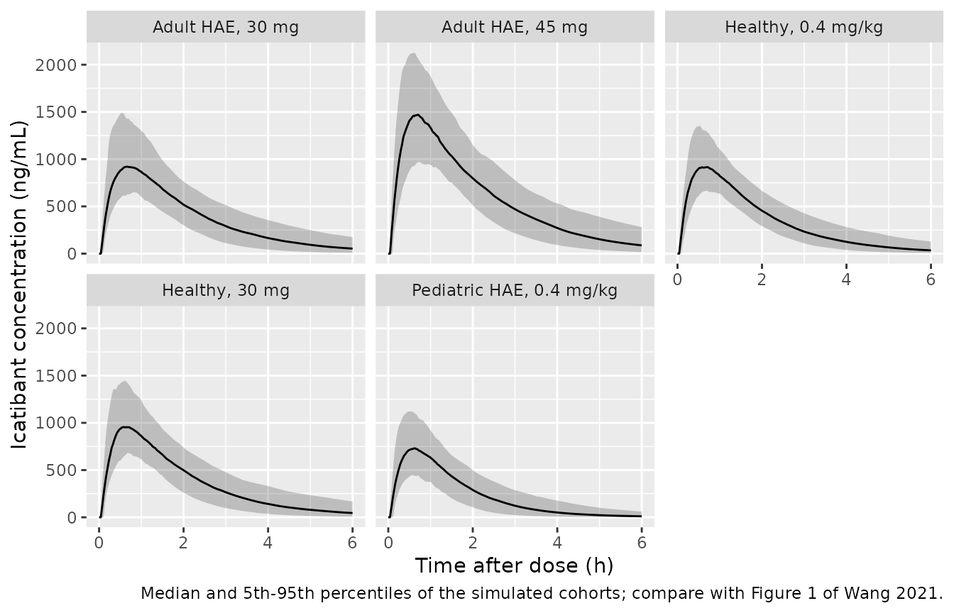
# Compare with Figure 1 of Wang 2021 (observed profiles by study; the
# 0-6 h window matches the pediatric sampling schedule).
sim |>
  group_by(treatment, time) |>
  summarise(
    Q05 = quantile(Cc, 0.05), Q50 = median(Cc), Q95 = quantile(Cc, 0.95),
    .groups = "drop"
  ) |>
  ggplot(aes(time, Q50)) +
  geom_ribbon(aes(ymin = Q05, ymax = Q95), alpha = 0.25) +
  geom_line() +
  facet_wrap(~treatment) +
  labs(
    x = "Time after dose (h)", y = "Icatibant concentration (ng/mL)",
    caption = "Median and 5th-95th percentiles of the simulated cohorts; compare with Figure 1 of Wang 2021."
  )

PKNCA validation

Table 3 of the paper reports Cmax and AUC0-6 derived from the final model with each subject’s actual dosing. The same quantities are computed here with PKNCA over 0-6 h.

sim_nca <- sim |>
  filter(!is.na(Cc)) |>
  select(id, time, Cc, treatment)
sim_nca <- bind_rows(
  sim_nca,
  sim_nca |> distinct(id, treatment) |> mutate(time = 0, Cc = 0)
) |>
  distinct(id, treatment, time, .keep_all = TRUE) |>
  arrange(id, treatment, time)

dose_df <- events |>
  filter(evid == 1) |>
  select(id, time, amt, treatment)

conc_obj <- PKNCA::PKNCAconc(sim_nca, Cc ~ time | treatment + id)
dose_obj <- PKNCA::PKNCAdose(dose_df, amt ~ time | treatment + id)
intervals <- data.frame(start = 0, end = 6, cmax = TRUE, auclast = TRUE)
nca_res <- PKNCA::pk.nca(PKNCA::PKNCAdata(conc_obj, dose_obj, intervals = intervals))

Comparison against published exposure

The published values are medians (Table 3). The comparison uses the median of the simulated cohort.

published <- tibble::tribble(
  ~treatment, ~cmax, ~auclast,
  "Pediatric HAE, 0.4 mg/kg", 747, 1288,
  "Healthy, 0.4 mg/kg", 1258, 2704,
  "Healthy, 30 mg", 915, 1941,
  "Adult HAE, 30 mg", 1254, 2975,
  "Adult HAE, 45 mg", 2222, 5565
)

cmp <- nlmixr2lib::ncaComparisonTable(
  simulated = nca_res,
  reference = published,
  by = "treatment",
  units = c(cmax = "ng/mL", auclast = "ng*h/mL"),
  tolerance_pct = 20
)
knitr::kable(cmp, caption = "Simulated vs. published (Table 3) median Cmax and AUC0-6. * differs from reference by >20%.")

Simulated vs. published (Table 3) median Cmax and AUC0-6. * differs from reference by >20%.

NCA parameter	treatment	Reference	Simulated	% diff
Cmax (ng/mL)	Pediatric HAE, 0.4 mg/kg	747	746	-0.1%
Cmax (ng/mL)	Healthy, 0.4 mg/kg	1260	927	-26.3%*
Cmax (ng/mL)	Healthy, 30 mg	915	965	+5.5%
Cmax (ng/mL)	Adult HAE, 30 mg	1250	934	-25.5%*
Cmax (ng/mL)	Adult HAE, 45 mg	2220	1480	-33.4%*
AUClast (ng*h/mL)	Pediatric HAE, 0.4 mg/kg	1290	1380	+7.1%
AUClast (ng*h/mL)	Healthy, 0.4 mg/kg	2700	2040	-24.7%*
AUClast (ng*h/mL)	Healthy, 30 mg	1940	2210	+14.0%
AUClast (ng*h/mL)	Adult HAE, 30 mg	2980	2310	-22.2%*
AUClast (ng*h/mL)	Adult HAE, 45 mg	5560	3540	-36.4%*

sim_med <- as.data.frame(nca_res) |>
  filter(PPTESTCD %in% c("cmax", "auclast")) |>
  group_by(treatment, PPTESTCD) |>
  summarise(sim = median(PPORRES), .groups = "drop") |>
  tidyr::pivot_wider(names_from = PPTESTCD, values_from = sim) |>
  inner_join(published, by = "treatment", suffix = c("_sim", "_pub")) |>
  mutate(
    cmax_pct = 100 * (cmax_sim / cmax_pub - 1),
    auc_pct = 100 * (auclast_sim / auclast_pub - 1)
  )
stopifnot(nrow(sim_med) == 5)

# The larger cohorts (pediatric, n = 31, and healthy 30 mg, n = 109) are the
# structural check: a mis-transcribed CL, volume, dose or unit moves both
# medians by tens of percent. Across three seeds the realised differences
# were -4 to +8% (Cmax) and +6 to +14% (AUC0-6); 20% leaves headroom over
# that spread.
big <-sim_med |> filter(treatment %in% c("Pediatric HAE, 0.4 mg/kg", "Healthy, 30 mg"))
stopifnot(nrow(big) == 2, all(abs(big$cmax_pct) < 20), all(abs(big$auc_pct) < 20))
sim_med |> select(treatment, cmax_pct, auc_pct)
#> # A tibble: 5 × 3
#>   treatment                cmax_pct auc_pct
#>   <chr>                       <dbl>   <dbl>
#> 1 Adult HAE, 30 mg          -25.5    -22.2 
#> 2 Adult HAE, 45 mg          -33.4    -36.4 
#> 3 Healthy, 0.4 mg/kg        -26.3    -24.7 
#> 4 Healthy, 30 mg              5.45    14.0 
#> 5 Pediatric HAE, 0.4 mg/kg   -0.142    7.12

The two large groups, pediatric patients (n = 31) and healthy adults given 30 mg (n = 109), are within 20% of Table 3. The other three groups run 22-36% below Table 3. These are not typical-value misses the model could correct. Table 3 summarises each observed subject’s post hoc prediction, and these groups had higher exposure than the model’s covariates explain:

• The healthy 0.4 mg/kg group (JE049-1102: young White men, about 31 mg per dose) has a published median AUC0-6 of 2704 ngh/mL. The healthy 30 mg group, given nearly the same dose, has 1941 ngh/mL. The final model has no study effect, so a population simulation cannot reproduce that 39% gap.
• The adult HAE groups have 4 patients each, so their published medians rest on very few subjects.

The pediatric and healthy 30 mg groups, together with the weight-band simulation below, are the validation. The other three rows are shown for completeness.

The paper also summarises this table as pediatric patients given 0.4 mg/kg having mean AUC0-6 and Cmax about 50% and 42% lower than adult patients given 30 mg. The simulated ratios below are closer to 1 because the simulated adult HAE cohort sits below its small published group, for the reasons above.

ratio <- sim_med |>
  filter(treatment %in% c("Pediatric HAE, 0.4 mg/kg", "Adult HAE, 30 mg")) |>
  arrange(treatment != "Pediatric HAE, 0.4 mg/kg")
c(
  AUC_ped_over_adult = ratio$auclast_sim[1] / ratio$auclast_sim[2],
  Cmax_ped_over_adult = ratio$cmax_sim[1] / ratio$cmax_sim[2]
)
#>  AUC_ped_over_adult Cmax_ped_over_adult 
#>           0.5964175           0.7989605

Weight-band dosing (Table S7 and Figure 4)

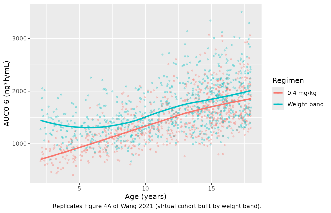
The paper simulated 6000 virtual pediatric patients and compared 0.4 mg/kg with a five-band regimen (10 mg for 12-25 kg, 15 mg for 26-40 kg, 20 mg for 41-50 kg, 25 mg for 51-65 kg, 30 mg above 65 kg). Here each band holds 150 virtual patients per regimen. Weights come from the same weight-for-age approximation as above; a draw that falls outside its band is discarded and redrawn rather than clipped.

bands <- data.frame(
  band = c("12-25", "26-40", "41-50", "51-65", ">65"),
  lo = c(12, 25, 40, 50, 65),
  hi = c(25, 40, 50, 65, 100),
  band_dose = c(10, 15, 20, 25, 30)
)

draw_band <- function(lo, hi, n_band) {
  out <- data.frame()
  while (nrow(out) < n_band) {
    age <- runif(2000, 2, 18)
    wt <- median_wt(age) * exp(rnorm(2000, 0, 0.18))
    keep <- wt > lo & wt <= hi
    out <- rbind(out, data.frame(AGE = age[keep], WT = wt[keep]))
  }
  out[seq_len(n_band), ]
}

n_band <- 150
band_events <- list()
for (i in seq_len(nrow(bands))) {
  covs <- draw_band(bands$lo[i], bands$hi[i], n_band) |>
    mutate(SEXF = rbinom(n_band, 1, 0.5), RACE_WHITE = 1, DIS_HAE_ACUTE = 1)
  off <- 10000L + (i - 1L) * 1000L
  band_events[[length(band_events) + 1]] <-
    make_cohort(covs, pmin(0.4 * covs$WT, 30), "0.4 mg/kg", off) |> mutate(band = bands$band[i])
  band_events[[length(band_events) + 1]] <-
    make_cohort(covs, bands$band_dose[i], "Weight band", off + 500L) |> mutate(band = bands$band[i])
}
band_events <- bind_rows(band_events)
stopifnot(!anyDuplicated(unique(band_events[, c("id", "time", "evid")])))

band_sim <- rxode2::rxSolve(mod, events = band_events, keep = c("treatment", "band", "AGE")) |>
  as.data.frame()

band_exp <- band_sim |>
  group_by(id, treatment, band, AGE) |>
  summarise(
    cmax = max(Cc),
    auc06 = sum(diff(time) * (head(Cc, -1) + tail(Cc, -1)) / 2),
    .groups = "drop"
  )

band_pub <- tibble::tribble(
  ~band, ~treatment, ~auc06_pub, ~cmax_pub,
  "12-25", "0.4 mg/kg", 869, 534,
  "26-40", "0.4 mg/kg", 1176, 672,
  "41-50", "0.4 mg/kg", 1474, 795,
  "51-65", "0.4 mg/kg", 1617, 839,
  ">65", "0.4 mg/kg", 1776, 868,
  "12-25", "Weight band", 1211, 747,
  "26-40", "Weight band", 1370, 775,
  "41-50", "Weight band", 1617, 867,
  "51-65", "Weight band", 1783, 924,
  ">65", "Weight band", 1836, 907
)

band_tab <- band_exp |>
  group_by(band, treatment) |>
  summarise(auc06_sim = median(auc06), cmax_sim = median(cmax), .groups = "drop") |>
  inner_join(band_pub, by = c("band", "treatment")) |>
  mutate(
    auc_pct = 100 * (auc06_sim / auc06_pub - 1),
    cmax_pct = 100 * (cmax_sim / cmax_pub - 1),
    band = factor(band, levels = bands$band)
  ) |>
  arrange(treatment, band)
stopifnot(nrow(band_tab) == 10)

band_tab |>
  dplyr::rename(
    "Weight band (kg)" = band, "Regimen" = treatment,
    "AUC0-6 sim" = auc06_sim, "AUC0-6 Table S7" = auc06_pub, "AUC0-6 % diff" = auc_pct,
    "Cmax sim" = cmax_sim, "Cmax Table S7" = cmax_pub, "Cmax % diff" = cmax_pct
  ) |>
  knitr::kable(digits = 0, caption = "Median AUC0-6 (ng*h/mL) and Cmax (ng/mL) by weight band: simulation vs Table S7 of Wang 2021.")

Median AUC0-6 (ng*h/mL) and Cmax (ng/mL) by weight band: simulation vs Table S7 of Wang 2021.

Weight band (kg)	Regimen	AUC0-6 sim	Cmax sim	AUC0-6 Table S7	Cmax Table S7	AUC0-6 % diff	Cmax % diff
12-25	0.4 mg/kg	921	545	869	534	6	2
26-40	0.4 mg/kg	1245	672	1176	672	6	0
41-50	0.4 mg/kg	1487	793	1474	795	1	0
51-65	0.4 mg/kg	1714	864	1617	839	6	3
>65	0.4 mg/kg	1835	932	1776	868	3	7
12-25	Weight band	1257	744	1211	747	4	0
26-40	Weight band	1430	813	1370	775	4	5
41-50	Weight band	1590	861	1617	867	-2	-1
51-65	Weight band	1913	970	1783	924	7	5
>65	Weight band	1921	964	1836	907	5	6

# Median of the per-band percent differences: centre of the distribution,
# not the extremes (see the note on cohort assertions in the package docs).
stopifnot(
  abs(median(band_tab$auc_pct)) < 15,
  abs(median(band_tab$cmax_pct)) < 20
)

# Published finding: the 10 mg band gives a median AUC0-6 39% higher than
# 0.4 mg/kg in the 12-25 kg band. That ratio is set mainly by the dose ratio,
# so it is a tight check on the band dosing logic.
r12 <- band_tab |> filter(band == "12-25")
ratio_12 <- r12$auc06_sim[r12$treatment == "Weight band"] / r12$auc06_sim[r12$treatment == "0.4 mg/kg"]
stopifnot(ratio_12 > 1.2, ratio_12 < 1.6)
ratio_12
#> [1] 1.364686

Table S7 is itself a simulation from the final model, so it is the most direct check on the packaged parameters. The band medians agree with it to within roughly 10%, and the 10 mg band again gives about 35-40% more exposure than 0.4 mg/kg in the lightest children, as the paper reports.

# Replicates Figure 4 of Wang 2021: simulated AUC0-6 versus age for the two regimens.
band_exp |>
  ggplot(aes(AGE, auc06, colour = treatment)) +
  geom_point(alpha = 0.3, size = 0.8) +
  geom_smooth(method = "loess", formula = y ~ x, se = FALSE) +
  labs(
    x = "Age (years)", y = "AUC0-6 (ng*h/mL)", colour = "Regimen",
    caption = "Replicates Figure 4A of Wang 2021 (virtual cohort built by weight band)."
  )

Assumptions and deviations

• BSV scale. Table 2 reports between-subject variability as a percentage for exponential random effects. The maintainers read these as coefficients of variation and converted them with omega^2 = log(CV^2 + 1). Reading them as sqrt(omega^2) instead would raise the variances, most for Clp/F (107.8%: 0.771 vs 1.162). No covariances are reported, so the random effects are independent.
• Categorical covariate effects. Table S5 footnote a states that sex, race and HAE-attack effects enter as exp(effect). Table 2 prints the multiplicative factor for the final model, so the model stores its logarithm. Table S5’s “Original” column is the full model (it still includes the HAE effect on Vc/F, which was then removed), so its coefficients differ slightly from Table 2; Table 2 is used throughout.
• HAE attack covariate. The paper describes the effect as applying to “pediatric patients who experienced an acute attack”. Table S2 shows the flag is also 1 for all 8 adult patients in JE049-2101. The covariate is therefore encoded as “dosed within 12 hours of an attack’s onset” for any age (DIS_HAE_ACUTE), not as a pediatric-only term.
• Race. The paper dichotomises race as White vs non-White; non-White pools Black or African American and Other. The canonical column is RACE_WHITE, so the effect enters on (1 - RACE_WHITE).
• Pediatric sample size. Table S1 says two patients younger than 6 years were excluded, leaving 29 pediatric patients. Table 1, Table S2 and Table 3 all count 31, including 2 aged 2-5 years, and that is the count used in the population metadata.
• Virtual cohorts. Pediatric weights come from an approximate median weight-for-age curve (CDC 2000 50th percentile, sexes pooled) with 18% log-normal spread. The paper used GAMLSS on growth-chart data, which is not reproduced here. The adult cohorts use the per-study summaries in Table S2. The weight-band simulation assumes all patients are White and dosed during an attack; the paper does not state the covariate settings it used.
• Table 3 comparison. Table 3 summarises individual (post hoc) predictions for the observed subjects. The simulations here draw new subjects, so only the medians of the larger groups are expected to agree closely.
• Residual error. The Methods describe additive, proportional and combined error structures. The final model in Table 2 lists only a proportional error (13.0%), and that is what the model uses.
• No correction or erratum to the article was found (EuropePMC search, 2026-09-28).