FOLFOX + panitumumab progression-free survival (Baaz 2023)
Source:vignettes/articles/Baaz_2023_panitumumab_folfox.Rmd
Baaz_2023_panitumumab_folfox.RmdModel and source
- Citation: Baaz M, Cardilin T, Jirstrand M. Model-based prediction of progression-free survival for combination therapies in oncology. CPT Pharmacometrics Syst Pharmacol. 2023;12(9):1227-1237. doi:10.1002/psp4.13003. Parameter estimates from Table 1; model code from the Monolix project in Data S1.
- Description (joint TGI / non-target progression): Joint tumor growth inhibition (TGI) and non-target-progression (NTP) time-to-event model for FOLFOX with or without panitumumab in RAS exon 2 wild-type metastatic colorectal cancer (Baaz 2023, PRIME study, n = 248). The sum of the largest target-lesion diameters (tumor_size, mm) grows exponentially at kge and is reduced by a dose-driven kill term, (kdrug_folfox * DOSE_FOLFOX_MGM2 + kdrug_panitumumab * DOSE_PANITUMUMAB_MGKG) * exp(-lambda * t), where the doses are the total dose per 14-day cycle and lambda is a resistance rate shared by both drugs. There is no PK model. The NTP hazard is linked to the tumor’s rate of change, h = max(e_dsld_haz * d(tumor_size)/dt + base_haz, 0), and its cumulative hazard gives the NTP survivor function sur. Time is in months from the start of treatment. The separately calibrated Weibull dropout model is modellib(‘Baaz_2023_panitumumab_folfox_dropout’).
- Description (dropout): Weibull time-to-dropout model for patients with RAS exon 2 wild-type metastatic colorectal cancer on FOLFOX with or without panitumumab (Baaz 2023, PRIME study, n = 248). Dropout (censoring without target or non-target progression) is independent of tumor response and of treatment; the hazard is h = (alfa_haz / te_haz) * (t / te_haz)^(alfa_haz - 1) with shape alfa_haz and characteristic time te_haz. Time is in months from the start of treatment. No random effects. Calibrated separately from the joint TGI / non-target-progression model modellib(‘Baaz_2023_panitumumab_folfox’); the paper combines the two to predict progression-free survival.
- Article: https://doi.org/10.1002/psp4.13003 (open access, PMC10508530)
Baaz 2023 builds a progression-free survival (PFS) model for FOLFOX with or without panitumumab from three parts:
- a tumor growth inhibition (TGI) model for the sum of the largest target diameters (SLD), driven by the dose per 14-day cycle of each drug, with a resistance term shared by both drugs;
- a time-to-event model for non-target progression (NTP: a new lesion,
unequivocal non-target progression, or death) whose hazard is linked to
the SLD rate of change,
h1 = max(alpha * dSLD/dt + beta, 0), estimated jointly with the TGI model in one Monolix project; - a Weibull model for dropout (censoring), calibrated separately.
PFS is then simulated: target progression (TP, a 20% and 5 mm
increase of SLD over its nadir) is read off a noisy simulated SLD series
at the visit times, NTP and dropout times are drawn from their survival
curves, and the earliest of the three sets the PFS time. The two Monolix
projects are packaged as two models,
Baaz_2023_panitumumab_folfox (parts 1-2) and
Baaz_2023_panitumumab_folfox_dropout (part 3); this article
reproduces the PFS algorithm on top of them.
Population
The models were fitted to the phase III PRIME study (FOLFOX4 with or without panitumumab 6 mg/kg every 2 weeks, first-line metastatic colorectal cancer), obtained via Project Data Sphere. After excluding patients with a RAS exon 2 mutation or only one SLD measurement, 127 FOLFOX and 121 FOLFOX + panitumumab patients remained (Baaz 2023 Methods). SLD was assessed about every 2 months. Table S1 describes the whole randomised PRIME arms (325 and 331 patients): median age 61-62 years (range 27-85), 62-67% male, 91-93% White, ECOG 0-1 in 94%, colon primary in 65-66%, liver metastases in 86-88%. The external validation arm is panitumumab monotherapy from the ASPECCT study (Table S1: 188 patients, median age 60.5 years).
str(readModelDb("Baaz_2023_panitumumab_folfox")()$population)
#> List of 11
#>  $ species       : chr "human"
#>  $ n_subjects    : int 248
#>  $ n_studies     : int 1
#>  $ age_range     : chr "27-85 years (whole PRIME population)"
#>  $ age_median    : chr "61-62 years by arm (whole PRIME population)"
#>  $ sex_female_pct: num 35
#>  $ race_ethnicity: Named num 92
#>   ..- attr(*, "names")= chr "White"
#>  $ disease_state : chr "metastatic colorectal cancer, RAS exon 2 wild-type, first-line treatment"
#>  $ dose_range    : chr "FOLFOX4 every 2 weeks (oxaliplatin 85 mg/m^2 day 1; leucovorin 200 mg/m^2 days 1-2; 5-FU 400 mg/m^2 bolus then "| __truncated__
#>  $ regions       : chr "multinational (56-60% Western Europe, Canada, Australia)"
#>  $ notes         : chr "PRIME phase III study data obtained via Project Data Sphere. Patients with a RAS exon 2 mutation or only one SL"| __truncated__
Source trace
| Equation / parameter | Value | Source location |
|---|---|---|
lrbase (SLD0) |
log(123) mm | Table 1 |
lkge (kg) |
log(0.074) 1/month | Table 1 |
lkdrug_folfox (aFOLFOX) |
log(2.0e-4) m^2/(mg month) | Table 1 |
lkdrug_panitumumab (aPani) |
log(7.3e-3) kg/(mg month) | Table 1 |
llambda (gamma) |
log(0.18) 1/month | Table 1; Methods: one gamma for both drugs |
e_dsld_haz (alpha) |
0.0041 1/mm | Table 1 |
lbase_haz (beta) |
log(0.035) 1/month | Table 1 |
etalrbase, etalkge,
etalkdrug_folfox, etallambda
|
0.76^2, 0.53^2, 0.41^2, 1.06^2 | Table 1 ‘BSV’ column (Monolix omega = SD of eta); diagonal (Methods) |
addSd (s1) |
2.27 mm | Table 1 and footnote |
propSd (s2) |
0.15 | Table 1 and footnote |
lalfa_haz (k) |
log(1.50) | Table 1 |
lte_haz (lambda) |
log(36) month | Table 1 |
d/dt(tumor_size) = kg*SLD - (aFOLFOX*D_FOLFOX + aPani*D_Pani)*exp(-gamma*t)*SLD |
n/a | Methods TGI equations; Data S1 (atot,
ddt_SLD) |
| growth set to 0 when SLD > 1e6 mm | n/a | Data S1 |
haz_ntp = max(alpha*dSLD/dt + beta, 0) |
n/a | Methods h1; Data S1 |
haz_drop = (k/lambda)*(t/lambda)^(k-1) |
n/a | Methods h2; Data S1 Weibull model |
DOSE_FOLFOX_MGM2 = 1285 |
mg/m^2 per cycle | Not printed; selected against Figure S1 below |
DOSE_PANITUMUMAB_MGKG = 6 |
mg/kg per cycle | Methods |
Structural checks
mod <- readModelDb("Baaz_2023_panitumumab_folfox")
mod_drop <- readModelDb("Baaz_2023_panitumumab_folfox_dropout")
ui <- rxode2::rxode(mod)
#> ℹ parameter labels from comments will be replaced by 'label()'
th <- ui$theta

kg <- exp(th[["lkge"]])
gam <- exp(th[["llambda"]])
sld0 <- exp(th[["lrbase"]])
a_folfox <- exp(th[["lkdrug_folfox"]])
a_pani <- exp(th[["lkdrug_panitumumab"]])

# Typical-value SLD has a closed form:
# SLD(t) = SLD0 * exp(kg*t - (a*D/gamma) * (1 - exp(-gamma*t))).
sld_closed <- function(t, kill0) {
  sld0 * exp(kg * t - kill0 / gam * (1 - exp(-gam * t)))
}

ev_typ <- tidyr::expand_grid(
  id = 1:2,
  time = c(0, 1, 2, 4, 6, 8, 12, 24)
) |>
  mutate(
    evid = 0,
    cmt = "tumor_size",
    DOSE_FOLFOX_MGM2 = 1285,
    DOSE_PANITUMUMAB_MGKG = ifelse(id == 1, 0, 6)
  )
# rxSolve output already carries the covariate columns.
typ <- rxode2::rxSolve(rxode2::zeroRe(mod), ev_typ, returnType = "data.frame") |>
  mutate(
    kill0 = a_folfox * DOSE_FOLFOX_MGM2 + a_pani * DOSE_PANITUMUMAB_MGKG,
    closed = sld_closed(time, kill0),
    rel_err = abs(tumor_size / closed - 1)
  )
#> ℹ parameter labels from comments will be replaced by 'label()'
#> ℹ omega/sigma items treated as zero: 'etalrbase', 'etalkge', 'etalkdrug_folfox', 'etallambda'
#> Warning: multi-subject simulation without without 'omega'
# Same parameters on both sides: the difference is pure ODE-solver error.
stopifnot(max(typ$rel_err) < 1e-4)
Two values quoted in the Discussion follow from Table 1:
- Tumor doubling time
log(2) / kg= 9.37 months; the paper quotes “~9.6 months” (0.074 is a rounded estimate; 9.6 months would correspond to kg = 0.072). - The paper’s “estimate of 0.33” for gamma is not the Table 1 median
(0.18). It matches the population mean of the log-normal gamma
when the Table 1 BSV is read as the standard deviation of eta,
0.18 * exp(1.06^2 / 2)= 0.316, which supports that reading.
The dropout model has a closed-form survivor function
S(t) = exp(-(t/lambda)^k):
FOLFOX dose per cycle (Figure S1)
The PD model is driven by “the total dose per cycle (14 days)”, with the three FOLFOX drugs’ doses combined, but the resulting number is not printed and the Monolix code in Data S1 estimates the per-month rate directly. Two readings of the FOLFOX4 schedule in the Methods are possible:
- each listed amount once: 85 + 200 + 400 + 600 = 1285 mg/m^2;
- the full two-day cycle (leucovorin and both 5-FU doses on days 1 and 2): 85 + 2 * (200 + 400 + 600) = 2485 mg/m^2.
They differ by a factor of almost two in the FOLFOX kill rate. Figure S1 (the SLD VPC) decides between them: early in treatment, before dropout and progression thin the observed population, the observed median SLD falls from about 135 mm to about 100 mm at 2 months and about 85 mm at 4 months in the FOLFOX arm (values read by eye from Figure S1).
ratio_typ <- function(t, d_folfox) {
  sld_closed(t, a_folfox * d_folfox) / sld0
}
dose_tab <- tibble(time = c(2, 4, 6, 8)) |>
  mutate(
    `Figure S1 observed median / baseline (by eye)` = c(0.74, 0.63, 0.58, 0.52),
    `D = 1285 mg/m^2` = ratio_typ(time, 1285),
    `D = 2485 mg/m^2` = ratio_typ(time, 2485)
  )
knitr::kable(dose_tab, digits = 2,
caption = "Typical SLD / baseline in the FOLFOX arm.")| time | Figure S1 observed median / baseline (by eye) | D = 1285 mg/m^2 | D = 2485 mg/m^2 |
|---|---|---|---|
| 2 | 0.74 | 0.75 | 0.50 |
| 4 | 0.63 | 0.65 | 0.33 |
| 6 | 0.58 | 0.61 | 0.25 |
| 8 | 0.52 | 0.61 | 0.22 |
# Deterministic: the per-administration sum reproduces the early VPC decline,
# the doubled cycle total predicts a shrinkage the data do not show.
stopifnot(
  abs(ratio_typ(2, 1285) - 0.74) < 0.08,
  abs(ratio_typ(4, 1285) - 0.63) < 0.08,
  ratio_typ(2, 2485) < 0.55
)
1285 mg/m^2 is used throughout. A stochastic check against the Figure S1 percentiles (simulated without dropout or progression, so only the early part is comparable with the observed curves):
set.seed(2023)
rxode2::rxSetSeed(2023)
n_arm <- 200
arms <- tibble::tribble(
  ~arm, ~DOSE_FOLFOX_MGM2, ~DOSE_PANITUMUMAB_MGKG,
  "FOLFOX", 1285, 0,
  "FOLFOX + panitumumab", 1285, 6,
  "Panitumumab", 0, 6
)
sim_grid <- seq(0, 48, by = 0.1)
make_cohort <- function(arm_row, id_offset) {
  tidyr::expand_grid(id = id_offset + seq_len(n_arm), time = sim_grid) |>
    mutate(
      evid = 0,
      cmt = "tumor_size",
      arm = arm_row$arm,
      DOSE_FOLFOX_MGM2 = arm_row$DOSE_FOLFOX_MGM2,
      DOSE_PANITUMUMAB_MGKG = arm_row$DOSE_PANITUMUMAB_MGKG
    )
}
events <- dplyr::bind_rows(lapply(seq_len(nrow(arms)), function(i) {
  make_cohort(arms[i, ], (i - 1L) * n_arm)
}))
stopifnot(!anyDuplicated(events[, c("id", "time")]))

# A fast-growing draw can reach the 1e6 mm growth cap of the source code within
# 48 months; the step change in dSLD/dt at the cap needs more solver steps than
# the default allows.
sim <- rxode2::rxSolve(mod, events, keep = "arm", returnType = "data.frame",
                       maxsteps = 1e6)
#> ℹ parameter labels from comments will be replaced by 'label()'
stopifnot(!anyNA(sim$tumor_size))
obs_s1 <- tibble::tribble(
  ~arm, ~time, ~sld,
  "FOLFOX", 0, 135, "FOLFOX", 2, 100, "FOLFOX", 4, 85, "FOLFOX", 6, 78,
  "FOLFOX", 8, 70,
  "FOLFOX + panitumumab", 0, 150, "FOLFOX + panitumumab", 3, 85,
  "FOLFOX + panitumumab", 8, 65
)
sim |>
  filter(arm != "Panitumumab", time <= 12, abs(time - round(time)) < 1e-8) |>
  group_by(arm, time) |>
  summarise(
    p10 = quantile(tumor_size, 0.1),
    p50 = quantile(tumor_size, 0.5),
    p90 = quantile(tumor_size, 0.9),
    .groups = "drop"
  ) |>
  ggplot(aes(time, p50)) +
  geom_ribbon(aes(ymin = p10, ymax = p90), alpha = 0.25, fill = "steelblue") +
  geom_line(colour = "steelblue") +
  geom_point(data = obs_s1, aes(time, sld), colour = "black") +
  facet_wrap(~arm) +
  labs(x = "Time (months)", y = "SLD (mm)",
       title = "Simulated 10th / 50th / 90th SLD percentiles",
       caption = "Points: observed medians read by eye from Figure S1 of Baaz 2023.")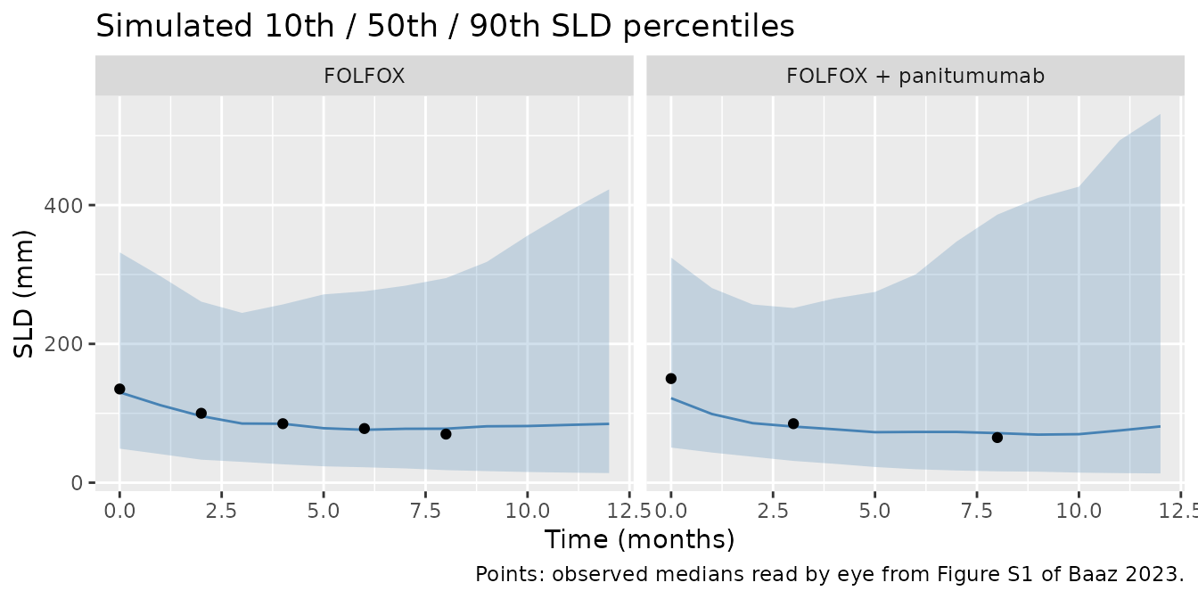
Progression-free survival (Figure 3, Table 2)
The PFS algorithm of the Methods is applied to the simulated cohort: visits every 2 months, TP when an SLD value is at least 20% and 5 mm above the nadir of the earlier visits (baseline included), NTP and dropout times drawn by inverting each subject’s cumulative hazard, and the earliest event sets the PFS time; dropout censors. Follow-up is cut at 48 months. Panitumumab monotherapy is the paper’s external prediction of ASPECCT, with PRIME-like patients assumed.
The paper’s TP rule is applied to “time series, including measurement
noise”, but how the noise enters the nadir is not specified, and the
result is sensitive to it: with s1 = 2.27 mm and s2 = 0.15, a single
noisy reading can cross the 20% threshold on its own. Both bounding
cases are therefore shown: TP read from the simulated observation
sim (model residual error) and from the noise-free
tumor_size.
visits <- seq(0, 48, by = 2)
drop_cum <- sim_drop$cumhaz

first_tp <- function(y) {
  for (j in seq_along(y)[-1]) {
    nadir <- min(y[seq_len(j - 1)])
    if (y[j] >= 1.2 * nadir && y[j] - nadir >= 5) {
      return(visits[j])
    }
  }
  Inf
}
first_crossing <- function(time, cumhaz, e) {
  k <- which(cumhaz >= e)[1]
  if (is.na(k)) Inf else time[k]
}
pfs_subject <- function(d, noisy, e_ntp, e_drop) {
  at_visit <- d[match(round(visits, 6), round(d$time, 6)), ]
  ttp <- first_tp(if (noisy) at_visit$sim else at_visit$tumor_size)
  tntp <- first_crossing(d$time, d$cumhaz, e_ntp)
  tdo <- first_crossing(drop_grid, drop_cum, e_drop)
  tt <- c(TP = ttp, NTP = tntp, Dropout = tdo, Administrative = 48)
  first <- names(tt)[which.min(tt)]
  tibble(time = min(tt), status = as.integer(first %in% c("TP", "NTP")),
         type = first)
}

ids <- unique(sim$id)
e_ntp <- stats::rexp(length(ids))
e_drop <- stats::rexp(length(ids))
sim_by_id <- split(sim, sim$id)
pfs <- dplyr::bind_rows(lapply(c(TRUE, FALSE), function(noisy) {
  dplyr::bind_rows(lapply(seq_along(ids), function(i) {
    d <- sim_by_id[[as.character(ids[i])]]
    pfs_subject(d, noisy, e_ntp[i], e_drop[i]) |>
      mutate(id = ids[i], arm = d$arm[1])
  })) |>
    mutate(tp_reading = if (noisy) "noisy SLD (sim)" else "noise-free SLD")
}))
km <- pfs |>
  group_by(arm, tp_reading) |>
  group_modify(function(d, key) {
    fit <- survival::survfit(survival::Surv(time, status) ~ 1, data = d)
    tibble(time = c(0, fit$time), surv = c(1, fit$surv))
  }) |>
  ungroup() |>
  mutate(arm = factor(arm, levels = arms$arm))
ggplot(km, aes(time, surv, colour = tp_reading)) +
  geom_step() +
  facet_wrap(~arm, scales = "free_x") +
  labs(x = "Time (months)", y = "Progression-free survival", colour = "TP read from",
       caption = "Replicates the median prediction of Figure 3 of Baaz 2023.") +
  theme(legend.position = "bottom")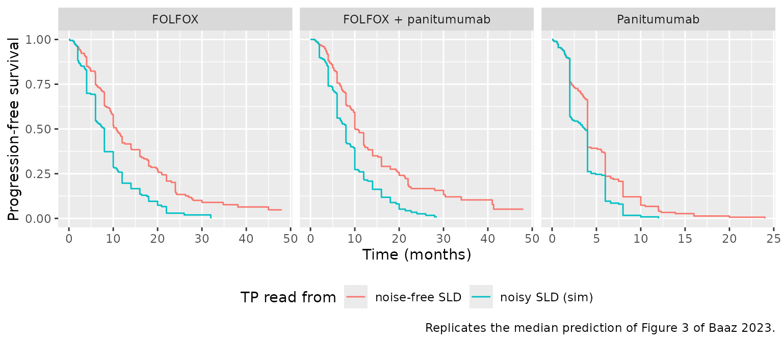
km_median <- function(d) {
  fit <- survival::survfit(survival::Surv(time, status) ~ 1, data = d)
  unname(summary(fit)$table["median"])
}
pfs_tab <- pfs |>
  group_by(arm, tp_reading) |>
  group_modify(function(d, key) {
    tibble(
      median = km_median(d),
      TP = mean(d$type == "TP"),
      NTP = mean(d$type == "NTP"),
      Dropout = mean(d$type == "Dropout")
    )
  }) |>
  ungroup()
paper <- tibble::tribble(
  ~arm, ~paper_median, ~paper_split,
  "FOLFOX", "8.5 (6.9-10.9)", "44 / 35 / 21",
  "FOLFOX + panitumumab", "9.1 (7.2-11.8)", "48 / 32 / 19",
  "Panitumumab", "4.7 (4.2-7.0)", "not reported"
)
pfs_tab |>
  left_join(paper, by = "arm") |>
  mutate(split = sprintf("%.0f / %.0f / %.0f", 100 * TP, 100 * NTP, 100 * Dropout)) |>
  select(arm, tp_reading, median, paper_median, split, paper_split) |>
  dplyr::rename(
    Arm = arm,
    `TP read from` = tp_reading,
    `Simulated median PFS (months)` = median,
    `Paper predicted median (95% CI)` = paper_median,
    `Simulated TP / NTP / dropout (%)` = split,
    `Paper virtual TP / NTP / dropout (%)` = paper_split
  ) |>
knitr::kable(digits = 1)| Arm | TP read from | Simulated median PFS (months) | Paper predicted median (95% CI) | Simulated TP / NTP / dropout (%) | Paper virtual TP / NTP / dropout (%) |
|---|---|---|---|---|---|
| FOLFOX | noise-free SLD | 10.7 | 8.5 (6.9-10.9) | 38 / 40 / 22 | 44 / 35 / 21 |
| FOLFOX | noisy SLD (sim) | 8.0 | 8.5 (6.9-10.9) | 67 / 19 / 14 | 44 / 35 / 21 |
| FOLFOX + panitumumab | noise-free SLD | 10.1 | 9.1 (7.2-11.8) | 40 / 32 / 28 | 48 / 32 / 19 |
| FOLFOX + panitumumab | noisy SLD (sim) | 8.0 | 9.1 (7.2-11.8) | 64 / 21 / 16 | 48 / 32 / 19 |
| Panitumumab | noise-free SLD | 4.0 | 4.7 (4.2-7.0) | 64 / 28 / 8 | not reported |
| Panitumumab | noisy SLD (sim) | 3.7 | 4.7 (4.2-7.0) | 73 / 22 / 4 | not reported |
med <- function(a, r) pfs_tab$median[pfs_tab$arm == a & pfs_tab$tp_reading == r]
stopifnot(nrow(pfs_tab) == 6L)
stopifnot(
  # FOLFOX-containing arms: the paper's predicted medians (8.5 and 9.1
  # months) lie between the two TP readings; a wrong dose or a mis-scaled
  # rate moves these by several months. Realised medians over three seeds
  # and two thread counts: 6.0-8.0 (noisy) and 10.0-12.0 (noise-free).
  all(c(med("FOLFOX", "noisy SLD (sim)"), med("FOLFOX + panitumumab", "noisy SLD (sim)")) > 4),
  all(c(med("FOLFOX", "noise-free SLD"), med("FOLFOX + panitumumab", "noise-free SLD")) < 15),
  # Panitumumab alone barely offsets growth (aPani * 6 = 0.044 < kg = 0.074):
  # PFS is short, as the paper predicts.
  med("Panitumumab", "noise-free SLD") < 6.5,
  med("Panitumumab", "noise-free SLD") < med("FOLFOX", "noise-free SLD") - 2
)
The paper’s predicted medians (8.5 and 9.1 months, Table 2 “All”) sit between the noisy and the noise-free TP readings. The noise-free reading gives roughly the paper’s virtual-patient event split for the FOLFOX arm (44% TP, 35% NTP, 21% dropout), while reading TP from noisy values shifts events towards TP and shortens PFS; the paper’s own implementation evidently lies in between. With 200 patients per arm and visits every 2 months, the simulated medians move by up to two months between random draws. The panitumumab monotherapy prediction comes out at about 3-4 months, somewhat below the paper’s 4.7 months (95% interval 4.2-7.0; 4.8 in the Discussion) and near the lower end of that interval. The ASPECCT visit schedule, which the paper does not give, affects this arm, and in it most events are TP, so the TP reading matters less than in the FOLFOX arms.
The truncated-data recalibrations of Figure 4 and the hazard ratios of Table 2 use re-estimated parameter sets that the paper does not report, so they are not reproduced.
NCA
Not applicable: the models have no pharmacokinetic component. The drugs act through their dose per cycle, so there are no concentrations for PKNCA to summarise; the validation above uses the closed-form SLD and dropout solutions and the paper’s PFS predictions instead.
Assumptions and deviations
-
FOLFOX dose per cycle. Not printed in the paper;
1285 mg/m^2 (each FOLFOX4 amount counted once) reproduces the early
decline of the Figure S1 VPC and is used here, while the full two-day
total of 2485 mg/m^2 does not. Users supplying a dose must use the same
convention, because the model is linear in
DOSE_FOLFOX_MGM2. -
BSV scale. Table 1 “BSV” is read as the Monolix
omega, the standard deviation of eta, and squared for
ini(). The Discussion’s mean gamma of 0.33 supports this reading. -
Residual error form. The paper states “an additive
and a proportional term” without the combination rule; the Monolix
default
combined1(SD = s1 + s2 * f) is encoded. - Two model files. The joint TGI / NTP model and the dropout model were separate Monolix projects (Data S1) and are packaged separately; the PFS combination is an algorithm, reproduced above, not a model equation.
-
Covariate analysis not encoded. Table 3 (and Table
S2, the Monolix automated builder) reports covariate weights on SLD0,
kg, gamma and aFOLFOX in
theta_i = theta_m * exp(eta_i + Z_i * w). The covariate units and centering values are not reported. Read uncentered as printed, the hemoglobin and lesion-count terms alone move the typical baseline SLD by tens of percent away from the observed baseline in Figure S1, and the paper’s PFS predictions all use the covariate-free model. The weights are recorded in the model’scovariatesDataExcludedmetadata. - Figure 4 and Table 2 hazard ratios. Based on re-estimated (truncated-data) parameter sets that are not reported; not reproduced.
-
Doubling time. Table 1 gives
log(2) / 0.074= 9.4 months against the Discussion’s “~9.6 months”; the difference is rounding of kg. - Panitumumab monotherapy population. As in the paper, PRIME-like patients are assumed for the ASPECCT prediction.