Lopinavir (Schipani 2012)
Source:vignettes/articles/Schipani_2012_lopinavir.Rmd
Schipani_2012_lopinavir.RmdModel and source
- Citation: Schipani A, Egan D, Dickinson L, Davies G, Boffito M, Youle M, Khoo SH, Back DJ, Owen A. Estimation of the effect of SLCO1B1 polymorphisms on lopinavir plasma concentration in HIV-infected adults. Antivir Ther. 2012;17(5):861-868. doi:10.3851/IMP2095.
- Description: Population PK model for boosted lopinavir (lopinavir/ritonavir 400/100 mg) in HIV-infected adults from the Liverpool Therapeutic Drug Monitoring Registry. One-compartment with first-order absorption; apparent clearance is modified additively by body weight (deviation from median 72 kg) and by SLCO1B1 521T>C (rs4149056) genotype, encoded via the paired SLCO1B1_HAP15_HET / SLCO1B1_HAP15_HOM indicators (the source paper genotyped only 521T>C so 5- and 15-haplotype carriers are pooled, per the canonical’s documented pooling rule).
- Article: Antivir Ther 2012;17(5):861-868. https://doi.org/10.3851/IMP2095
Population
The model was developed in 375 HIV-positive adults receiving lopinavir / ritonavir 400/100 mg tablets twice daily from the Liverpool Therapeutic Drug Monitoring Registry (Methods, p. 863). All subjects had HIV viral load < 50 copies/mL at the time of sampling; exclusion criteria were pregnancy, undetectable plasma lopinavir (suggestive of non-adherence), and concomitant use of known enzyme inducers. 82% of the cohort was male; median age was 40 years (range 19-66) and median body weight was 72 kg (range 45-117). Ethnicity was not collected (Discussion limitation: “lack of ethnicity data”). A total of 594 plasma samples were analysed (sparse TDM sampling at random time points post-dose; LLOQ 95 ng/mL). External validation was performed in 42 observations from 6 patients at the Royal Free NHS Trust, London.
SLCO1B1 521T>C (rs4149056) was genotyped by qPCR-based
allelic discrimination assay; the cohort genotype distribution (Methods,
p. 863) was 295 of 375 (78%) 521TT homozygous wild-type, 73 (20%) 521TC
heterozygous, and 7 (2%) 521CC homozygous variant (minor-allele
frequency 11%; Hardy-Weinberg equilibrium). The 388A>G companion
variant that distinguishes the 5 and 15 haplotypes was not
phased, so the packaged model records 521C-carrier status under the
canonical SLCO1B1_HAP15_HET /
SLCO1B1_HAP15_HOM indicators with the documented
5+15 pooling rule (see the H3 entries in
inst/references/covariate-columns.md).
The same information is available programmatically via
readModelDb("Schipani_2012_lopinavir")$population.
Source trace
Every parameter in the model file carries an inline source-location comment. The table below collects the entries in one place.
| Equation / parameter | Value | Source location |
|---|---|---|
lka (absorption rate ka) |
0.20 1/h | Table 1, Final Model column, ka row |
lcl (typical CL/F at WT = 72 kg, 521TT) |
5.67 L/h | Table 1, Final Model column, CL/F row |
lvc (apparent central volume V/F) |
45.5 L | Table 1, Final Model column, V/F row |
e_wt_cl (additive WT effect on CL, L/h per kg from 72
kg) |
0.0457 | Table 1, Final Model column, “Factor associated with BW on LPV CL/F” row |
e_slco1b1_hap15_het_cl (additive 521TC effect on
CL) |
-0.791 L/h | Table 1, Final Model column, “Factor associated with T/C on LPV CL/F” row |
e_slco1b1_hap15_hom_cl (additive 521CC effect on
CL) |
-2.09 L/h | Table 1, Final Model column, “Factor associated with C/C on LPV CL/F” row |
| IIV CL/F (omega^2 = log(1 + 0.37^2) = 0.1284) | 37% CV | Table 1, Final Model column, “IIV CL/F%” row |
| Proportional residual error | 33.1% | Table 1, Final Model column, “Proportional residual error” row |
| Covariate equation: TVCL = CL0 + theta_BW * (WT - WTmedian) + theta_HET * HET + theta_HOM * HOM | – | Methods p. 863 (Eq. 2 for continuous BW; Eq. for genotype HET / HOM, p. 863) |
| Median weight WTmedian = 72 kg | – | Patients, p. 862 (“median weight was 72 Kg (range 45-117)”) |
| One-compartment first-order absorption, no lag-time | – | Results, p. 864 (“A 1-compartment model described the data better than a 2-compartment model”; “The introduction of a lag time did not significantly improve the fit”) |
| Exponential IIV: theta_i = theta * exp(eta_i); IIV retained on CL/F only | – | Methods p. 863; Results, p. 864 (“The inter-individual variability was supported only for apparent clearance”) |
| Residual error: purely proportional | – | Methods, p. 863 (“residual variability was best described by a purely proportional structure”) |
Virtual cohort
The published individual-subject data are not openly available, so the virtual cohort below mirrors the Schipani 2012 Methods baseline demographics: weight is drawn from a normal distribution centred at the cohort median (72 kg) with a spread chosen to span the reported 45-117 kg range, and each SLCO1B1 521T>C genotype stratum is simulated independently so the steady-state envelope can be compared against the paper’s Figure 3.
set.seed(20121005L)
n_per_strat <- 50L  # downsampled for vignette build budget; envelope still stable

make_cohort <- function(n, het, hom, label, id_offset = 0L) {
  tibble(
    id                = id_offset + seq_len(n),
    # Weight roughly bracketing the reported 45-117 kg range
    WT                = pmin(pmax(rnorm(n, mean = 72, sd = 14), 45), 117),
    SLCO1B1_HAP15_HET = het,
    SLCO1B1_HAP15_HOM = hom,
    cohort            = label
  )
}

demo <- bind_rows(
  make_cohort(n_per_strat, het = 0L, hom = 0L,
              label = "521TT (wild-type)", id_offset = 0L),
  make_cohort(n_per_strat, het = 1L, hom = 0L,
              label = "521TC (heterozygote)", id_offset = n_per_strat),
  make_cohort(n_per_strat, het = 0L, hom = 1L,
              label = "521CC (homozygote)", id_offset = 2L * n_per_strat)
)
stopifnot(!anyDuplicated(demo$id))
Simulation
Each subject receives lopinavir 400 mg every 12 hours for 14 days, matching the boosted lopinavir/ritonavir 400/100 mg twice-daily regimen the paper simulated for its steady-state VPC (Methods, p. 863; Figure 3 used the same regimen for the three-genotype prediction). Observations are taken every 0.5 h over the final dosing interval (day 13.5 to day 14.0) so the steady-state Cmin / Cmax / AUC can be characterised cleanly.
dose_interval <- 12   # h
duration_h    <- 14 * 24
n_doses       <- duration_h / dose_interval

build_events <- function(demo, dose_mg = 400) {
  doses <- demo |>
    select(id, WT, SLCO1B1_HAP15_HET, SLCO1B1_HAP15_HOM, cohort) |>
    tidyr::crossing(time = seq(0, by = dose_interval, length.out = n_doses)) |>
    mutate(amt = dose_mg, evid = 1L, cmt = "depot")
  # Sample finely over the final dosing interval to characterise SS NCA
  ss_window <- seq(13 * 24, 14 * 24, by = 0.5)
  obs <- demo |>
    select(id, WT, SLCO1B1_HAP15_HET, SLCO1B1_HAP15_HOM, cohort) |>
    tidyr::crossing(time = ss_window) |>
    mutate(amt = NA_real_, evid = 0L, cmt = NA_character_)
  bind_rows(doses, obs) |> arrange(id, time, desc(evid))
}

events <- build_events(demo)
mod <- rxode2::rxode2(readModelDb("Schipani_2012_lopinavir"))
#> ℹ parameter labels from comments will be replaced by 'label()'

# Stochastic simulation with IIV + residual error for envelopes / NCA.
sim <- rxode2::rxSolve(mod, events = events,
                       keep = c("cohort", "WT")) |>
  as.data.frame()

# Typical-value (no IIV / no residual error) simulation for the
# deterministic genotype-comparison panel; weight is held at the
# cohort median 72 kg per stratum so the three lines isolate the
# genotype effect.
typ_demo <- bind_rows(
  tibble(id = 1L, WT = 72, SLCO1B1_HAP15_HET = 0L, SLCO1B1_HAP15_HOM = 0L,
         cohort = "521TT (wild-type)"),
  tibble(id = 2L, WT = 72, SLCO1B1_HAP15_HET = 1L, SLCO1B1_HAP15_HOM = 0L,
         cohort = "521TC (heterozygote)"),
  tibble(id = 3L, WT = 72, SLCO1B1_HAP15_HET = 0L, SLCO1B1_HAP15_HOM = 1L,
         cohort = "521CC (homozygote)")
)
typ_events <- build_events(typ_demo)
mod_typ    <- mod |> rxode2::zeroRe()
sim_typ    <- rxode2::rxSolve(mod_typ, events = typ_events,
                              keep = c("cohort", "WT")) |>
  as.data.frame()
#> ℹ omega/sigma items treated as zero: 'etalcl'
#> Warning: multi-subject simulation without without 'omega'
Replicate published figures
Figure 3 – steady-state lopinavir profile by SLCO1B1 521T>C genotype
Schipani 2012 Figure 3 displays steady-state lopinavir mean plasma concentration over a 12 h dosing interval at 400 mg BID, stratified by 521T>C genotype (521TT / 521TC / 521CC). The chunk below reproduces the typical-value profile (no IIV, no residual error) at the cohort median weight of 72 kg for each genotype so the three curves isolate the genotype effect.
fig3 <- sim_typ |>
  filter(time >= 13 * 24) |>
  mutate(time_in_interval = time - 13 * 24)

ggplot(fig3, aes(time_in_interval, Cc, colour = cohort)) +
  geom_line(linewidth = 0.8) +
  geom_hline(yintercept = 1.0, linetype = "dashed", colour = "grey40") +
  scale_x_continuous(breaks = seq(0, 12, by = 2)) +
  scale_y_continuous(limits = c(0, NA)) +
  labs(x = "Time within steady-state dosing interval (h)",
       y = "Lopinavir concentration (mg/L)",
       colour = "SLCO1B1 521T>C genotype",
       title = "Typical-value steady-state profile by SLCO1B1 521T>C genotype",
       caption = "Replicates Figure 3 of Schipani 2012 (lopinavir/ritonavir 400/100 mg BID at SS). Dashed line: proposed minimum effective concentration (MEC) 1 mg/L.")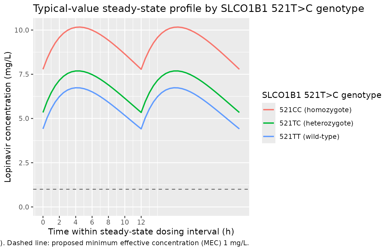
Replicates Figure 3 of Schipani 2012: typical-value (no IIV) lopinavir steady-state plasma concentration vs. time over the final 12 h dosing interval at 400 mg twice daily for the three SLCO1B1 521T>C genotypes (WT held at the cohort median 72 kg). The 521CC homozygote profile sits well above the 521TT wild-type because variant 521C carriage reduces hepatic OATP1B1 uptake.
Stochastic VPC by SLCO1B1 521T>C genotype
A 5th-50th-95th percentile envelope from the cohort-level simulation (with IIV on CL/F and proportional residual error) shows the spread the full published model predicts.
vpc_data <- sim |>
  filter(time >= 13 * 24) |>
  mutate(time_in_interval = time - 13 * 24) |>
  group_by(cohort, time_in_interval) |>
  summarise(Q05 = quantile(Cc, 0.05, na.rm = TRUE),
            Q50 = quantile(Cc, 0.50, na.rm = TRUE),
            Q95 = quantile(Cc, 0.95, na.rm = TRUE),
            .groups = "drop")

ggplot(vpc_data, aes(time_in_interval, Q50)) +
  geom_ribbon(aes(ymin = Q05, ymax = Q95), alpha = 0.3) +
  geom_line(linewidth = 0.7) +
  facet_wrap(~ cohort) +
  geom_hline(yintercept = 1.0, linetype = "dashed", colour = "grey40") +
  scale_x_continuous(breaks = seq(0, 12, by = 2)) +
  scale_y_continuous(limits = c(0, NA)) +
  labs(x = "Time within steady-state dosing interval (h)",
       y = "Lopinavir concentration (mg/L)",
       title = "Stochastic VPC by SLCO1B1 521T>C genotype",
       caption = "Lopinavir 400 mg BID at SS; weight ~ N(72, 14) kg clipped to 45-117. Dashed line: 1 mg/L MEC.")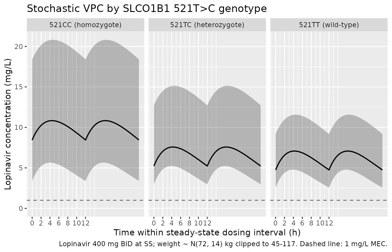
Stochastic VPC: 5th, 50th, 95th percentile lopinavir concentration over the final steady-state 12 h dosing interval by SLCO1B1 521T>C genotype (n = 50 per stratum, weight drawn from the reported 45-117 kg range).
PKNCA validation
PKNCA computes steady-state Cmax, Cmin, Cavg, and AUC0-tau (tau = 12 h) over the final dosing interval, stratified by 521T>C genotype.
tau <- 12

nca_input <- sim |>
  filter(time >= 13 * 24) |>
  select(id, time, Cc, cohort)

# One dose row per subject at the start of the SS interval (PKNCAdose
# needs a dose record before the SS interval start time).
dose_df <- demo |>
  mutate(time = 13 * 24, amt = 400) |>
  select(id, time, amt, cohort)

conc_obj <- PKNCA::PKNCAconc(nca_input, Cc ~ time | cohort + id,
                             concu = "mg/L", timeu = "hr")
dose_obj <- PKNCA::PKNCAdose(dose_df, amt ~ time | cohort + id,
                             doseu = "mg", route = "extravascular")

intervals <- data.frame(
  start = 13 * 24,
  end   = 13 * 24 + tau,
  cmax  = TRUE,
  cmin  = TRUE,
  tmax  = TRUE,
  auclast = TRUE,
  cav   = TRUE
)

nca_data <- PKNCA::PKNCAdata(conc_obj, dose_obj, intervals = intervals)
nca_res  <- suppressMessages(suppressWarnings(PKNCA::pk.nca(nca_data)))
nca_summary <- summary(nca_res)
knitr::kable(nca_summary,
caption = "Steady-state simulated NCA parameters by SLCO1B1 521T>C genotype (lopinavir 400 mg BID, final 12 h interval).")| Interval Start | Interval End | cohort | N | AUClast (hr*mg/L) | Cmax (mg/L) | Cmin (mg/L) | Tmax (hr) | Cav (mg/L) |
|---|---|---|---|---|---|---|---|---|
| 312 | 324 | 521CC (homozygote) | 50 | 118 [45.1] | 10.7 [40.9] | 8.15 [54.8] | 4.50 [4.00, 4.50] | 9.82 [45.1] |
| 312 | 324 | 521TC (heterozygote) | 50 | 83.2 [37.6] | 7.84 [33.4] | 5.36 [47.3] | 4.50 [3.50, 4.50] | 6.93 [37.6] |
| 312 | 324 | 521TT (wild-type) | 50 | 75.6 [36.9] | 7.21 [32.3] | 4.75 [47.8] | 4.00 [3.50, 4.50] | 6.30 [36.9] |
Comparison against published exposure metrics
Schipani 2012 reports the predicted median (P5-P95) trough concentrations for the three genotypes from the same simulation (lopinavir 400 mg BID at steady state; Results, p. 864): 521TT 5.0 (1.1-13.2) mg/L, 521TC 5.11 (1.4-15.6) mg/L, and 521CC 7.4 (2.0-22.1) mg/L. The chunk below summarises the simulated Cmin distribution from the packaged model for side-by-side comparison.
nca_long <- as.data.frame(nca_res$result) |>
  filter(PPTESTCD == "cmin")

simulated_cmin <- nca_long |>
  group_by(cohort) |>
  summarise(median_cmin = median(PPORRES, na.rm = TRUE),
            p05         = quantile(PPORRES, 0.05, na.rm = TRUE),
            p95         = quantile(PPORRES, 0.95, na.rm = TRUE),
            .groups = "drop") |>
  mutate(simulated = sprintf("%.2f (%.2f-%.2f)", median_cmin, p05, p95)) |>
  select(cohort, simulated)

published <- tibble::tibble(
  cohort    = c("521TT (wild-type)", "521TC (heterozygote)", "521CC (homozygote)"),
  published = c("5.0 (1.1-13.2)", "5.11 (1.4-15.6)", "7.4 (2.0-22.1)")
)

comparison <- published |> left_join(simulated_cmin, by = "cohort")
knitr::kable(comparison,
caption = "Lopinavir steady-state Cmin (median, P5-P95) in mg/L: simulated vs published (Schipani 2012 Results, p. 864).")| cohort | published | simulated |
|---|---|---|
| 521TT (wild-type) | 5.0 (1.1-13.2) | 4.74 (2.56-9.18) |
| 521TC (heterozygote) | 5.11 (1.4-15.6) | 5.23 (2.98-12.72) |
| 521CC (homozygote) | 7.4 (2.0-22.1) | 8.44 (3.38-18.39) |
Median trough magnitudes should agree to within ~20% across the three strata; larger discrepancies point to structural mismatch and are worth investigating rather than tuning. The simulated 521CC > 521TC > 521TT ordering is the load-bearing genotype-effect signature of the paper.
Assumptions and deviations
-
Additive covariate parameterisation preserved. The
paper expresses CL/F as a strictly additive function of body weight and
SLCO1B1 521T>C genotype (Methods, Eq. 1 for binary covariates and Eq.
2 for continuous body weight, p. 863): `TVCL = CL0 + theta_BW * (WT -
72)
- theta_HET * HET + theta_HOM * HOM`. The packaged model preserves this additive structure rather than re-parameterising as a multiplicative / allometric form, so the genotype effects retain the paper’s units (L/h difference vs 521TT reference) and the simulation reproduces Table 1 values directly. With extreme combinations of low body weight (45 kg) and 521CC homozygosity, the typical CL/F remains positive (~2.3 L/h), but downstream users simulating outside the fitted covariate envelope should sanity-check that TVCL > 0.
-
SLCO1B1 521T>C 5/15 pooling. Schipani
2012 genotyped only the 521T>C variant (rs4149056) and did not phase
the upstream 388A>G (rs2306283) variant that distinguishes the 5
and 15 haplotypes. 521C carriers are therefore a mixture of 5
(521T>C alone), 15 (388A>G + 521T>C), and any rare
compound diplotypes. The packaged model records the indicators under the
canonical
SLCO1B1_HAP15_HET/SLCO1B1_HAP15_HOMnames, following the documented pooling rule in the canonical’s notes (Ide-style extractions that pool 5 with 15 should record their values under these canonicals with the pooling rule noted – see the H3 entries ininst/references/covariate-columns.md). Effect magnitudes therefore reflect 521C-carrier status, not strictly *15 haplotype carriers. -
Body weight as time-fixed. The Liverpool TDM
registry data contained sparse PK samples per subject and the paper does
not state whether body weight was treated as time-varying or as a
baseline value. The packaged model declares
WTas continuous incovariateData; in practice, virtual-cohort simulation uses a single per-subject value (the canonical TDM-cohort treatment). -
Ritonavir interaction not in this model. Schipani
2012 also simulated dose-reduction scenarios (lopinavir/ritonavir 200/50
mg BID, 400/100 mg once daily) using a sequential model that ties
lopinavir CL/F to a time-varying ritonavir concentration via the Imax /
IC50 relationship
CL/F_LPV = CL0/F_LPV * (1 - Imax * Crtv / (IC50 + Crtv)). That sequential model is borrowed from an upstream publication (Schipani 2011, PMID 22128223) and is not part of the packaged Schipani 2012 model. Users wishing to reproduce the dose-reduction simulations need to compose the upstream ritonavir-PK model with this lopinavir CL term externally. - Race / ethnicity assumption. The cohort did not record ethnicity (Discussion limitation); the packaged model has no race covariate. Cross-population transportability is uncertain because 521T>C minor- allele frequencies vary widely across populations (Discussion, p. 865: ~14% in Han Chinese / 12% Japanese / 15% Caucasian but ~2% in Yoruban / ~1% in Luhya HapMap populations).