Miltefosine (Dorlo 2008)
Source:vignettes/articles/Dorlo_2008_miltefosine.Rmd
Dorlo_2008_miltefosine.RmdModel and source
- Citation: Dorlo TPC, van Thiel PPAM, Huitema ADR, Keizer RJ, de Vries HJC, Beijnen JH, de Vries PJ. Pharmacokinetics of miltefosine in Old World cutaneous leishmaniasis patients. Antimicrob Agents Chemother. 2008;52(8):2855-2860. doi:10.1128/AAC.00014-08.
- Description: Two-compartment population PK model with first-order oral absorption and linear elimination for miltefosine in 31 Dutch military personnel with Old World (Leishmania major) cutaneous leishmaniasis contracted in Afghanistan (Dorlo 2008), treated with oral miltefosine 50 mg three times daily (150 mg/day, median 1.76 mg/kg/day) for 28 days with post-treatment follow-up to a maximum of 202 days. CL/F, Vc/F, Q/F, and Vp/F are estimated apparent parameters; relative bioavailability F is unidentifiable from oral-only data and is structurally fixed at 1. Inter-individual variability is log-normal on ka, CL/F, and Vc/F (diagonal in this implementation; see Assumptions in the vignette for the unreported CL/Vc correlation noted by the authors). IIV on Q/F and Vp/F was not estimable from the data. Residual error is proportional (31.5% CV). No covariate effects were retained in the final model. This is the structural model later re-used as the base PK structure in Dorlo 2017 visceral-leishmaniasis miltefosine work.
- Article: https://doi.org/10.1128/AAC.00014-08
Population
The Dorlo 2008 model is a single-study population-PK analysis of oral
miltefosine in 31 Dutch military personnel and embedded civilians who
contracted Old World cutaneous leishmaniasis (Leishmania major) during
deployment in northern Afghanistan (ISAF Election Support Force). All
patients were treated at the Academic Medical Center, Amsterdam, on an
outpatient basis with 50 mg oral miltefosine (Impavido) three times
daily for 28 days (total 150 mg/day; median 1.76 mg/kg/day, IQR
1.69-1.92). The cohort had a median (IQR) age of 24 (23-29) years, body
weight 85 (78-89) kg, and height 184 (180-188) cm; 30 of 31 were male,
and 30 of 31 had received prior intralesional pentavalent antimony (SbV)
for the same lesions. Leishmaniasis was parasitologically confirmed in
all patients (microscopy plus PCR/NASBA genotyping in 27 of 31, all
confirming L. major). 382 plasma concentrations were analysed (median 13
samples per patient, range 9-20; LLOQ 4 ng/mL, all post-baseline samples
above LLOQ). The same information is available programmatically via
rxode2::rxode(readModelDb("Dorlo_2008_miltefosine"))$population.
Source trace
The per-parameter origin is recorded as a trailing in-file comment
next to each ini() entry in
inst/modeldb/specificDrugs/Dorlo_2008_miltefosine.R. The
table below collects them in one place for review.
| Equation / parameter | Value | Source location (Dorlo 2008) |
|---|---|---|
lka (ka) |
0.36 1/h x 24 = 8.64 1/day | Table 2 ‘Absorption rate (k_a) (h^-1)’ = 0.36 (RSE 10.1%) |
lcl (CL/F) |
3.87 L/day | Table 2 ‘Clearance (CL/F) (liters/day)’ = 3.87 (RSE 5.3%) |
lvc (Vc/F; paper V2/F) |
39.6 L | Table 2 ‘Volume of central compartment (V_2/F) (liters)’ = 39.6 (RSE 4.0%) |
lq (Q/F) |
0.0375 L/day | Table 2 ‘Intercompartmental clearance (Q/F) (liters/day)’ = 0.0375 (RSE 22.0%) |
lvp (Vp/F; paper V3/F) |
1.65 L | Table 2 ‘Volume of peripheral compartment (V_3/F) (liters)’ = 1.65 (RSE 12.4%) |
lfdepot |
log(1) FIXED | Methods ‘Pharmacokinetic data analysis’ paragraph 3: F unknown, parameters relative to F |
| Two-compartment ODE structure with first-order absorption | n/a | Results ‘Pharmacokinetic data analysis’ paragraph 3: ‘An open two-compartmental model with first-order absorption and linear elimination from the central compartment best fitted the data’ |
etalka |
log(1 + 0.242^2) = 0.0554 | Table 2 IIV ‘Absorption rate’ = 24.2% CV (RSE 63.3%) |
etalcl |
log(1 + 0.232^2) = 0.0511 | Table 2 IIV ‘Clearance’ = 23.2% CV (RSE 15.4%; footnote a: high correlation with V2/F IIV) |
etalvc |
log(1 + 0.183^2) = 0.0324 | Table 2 IIV ‘Volume of central compartment’ = 18.3% CV (RSE 25.0%; footnote a: high correlation with CL/F IIV) |
propSd |
0.315 | Table 2 ‘Residual variability (%)’ = 31.5 (RSE 6.4%) |
The first elimination half-life and terminal elimination half-life implied by the disposition parameters are:
cl <- 3.87 ; vc <- 39.6 ; q <- 0.0375 ; vp <- 1.65
kel <- cl / vc ; k12 <- q / vc ; k21 <- q / vp
ab  <- kel + k12 + k21
ab2 <- kel * k21
disc  <- sqrt(ab^2 - 4 * ab2)
alpha <- (ab + disc) / 2
beta  <- (ab - disc) / 2
data.frame(
  parameter = c("t1/2 (first / alpha)", "t1/2 (terminal / beta)"),
  predicted_days = round(log(2) / c(alpha, beta), 2),
  paper_days     = c(7.05, 30.9)
)
#>                parameter predicted_days paper_days
#> 1   t1/2 (first / alpha)           7.00       7.05
#> 2 t1/2 (terminal / beta)          30.88      30.90
These reproduce the values reported in the Results paragraph ‘Pharmacokinetic data analysis’ (first half-life 7.05 days, terminal half-life 30.9 days).
Virtual cohort
Original observed concentrations are not publicly available. We simulate a cohort that mirrors the published trial arm: 200 virtual subjects given 50 mg of miltefosine three times daily for 28 days, with concentration sampling extending to day 210 to bracket the post-treatment observation window described in the paper (samples collected up to 5-6 months / approximately 202 days after the start of treatment).
set.seed(2008)

n_subj      <- 200L
dose_mg     <- 50           # 50 mg per dose (Methods 'Protocol')
ii_day      <- 1 / 3        # three doses per day (50 mg t.i.d.)
n_days      <- 28           # 28-day treatment course
follow_days <- 210          # post-treatment follow-up to ~day 202 + buffer

events <- rxode2::et() |>
  rxode2::et(amt = dose_mg, ii = ii_day, until = n_days, cmt = "depot") |>
  rxode2::et(seq(0, follow_days, by = 0.5)) |>
  rxode2::et(id = seq_len(n_subj))
events$treatment <- "Miltefosine 50 mg TID, 28 days"
Simulation
mod <- readModelDb("Dorlo_2008_miltefosine")
sim <- rxode2::rxSolve(mod, events = events, keep = c("treatment"))
sim_df <- as.data.frame(sim)
For a deterministic typical-value replication (no between-subject variability), zero the random effects:
Replicate published figures
Figure 1 – Visual predictive check of miltefosine plasma concentrations
The paper’s Figure 1 shows individual observed concentrations from all 31 patients overlaid on the model’s 90% prediction interval and median predicted concentration over the 28-day treatment course and the follow-up window. Concentrations are reported in ng/mL; the model file uses ug/mL internally (mg/L), so we multiply by 1000 for display.
sim_vpc <- sim_df |>
  dplyr::group_by(time) |>
  dplyr::summarise(
    Q05 = quantile(Cc, 0.05, na.rm = TRUE) * 1000,
    Q50 = quantile(Cc, 0.50, na.rm = TRUE) * 1000,
    Q95 = quantile(Cc, 0.95, na.rm = TRUE) * 1000,
    .groups = "drop"
  )

ggplot(sim_vpc, aes(time, Q50)) +
  geom_ribbon(aes(ymin = Q05, ymax = Q95), alpha = 0.25) +
  geom_line() +
  scale_y_log10(limits = c(1, 1e5)) +
  labs(x = "Time after start of treatment (days)",
       y = "Miltefosine plasma concentration (ng/mL)",
       title = "Figure 1 -- Simulated VPC of miltefosine in cutaneous leishmaniasis patients",
       caption = paste(
         "Replicates Figure 1 of Dorlo 2008.",
         "Shaded band: simulated 90% prediction interval (5th-95th percentile).",
         "Solid line: simulated median.",
         "Source paper plots observations vs. a 2,000-subject VPC of the same model."
       ))
#> Warning in scale_y_log10(limits = c(1, 1e+05)): log-10 transformation introduced infinite values.
#> log-10 transformation introduced infinite values.
#> log-10 transformation introduced infinite values.
#> log-10 transformation introduced infinite values.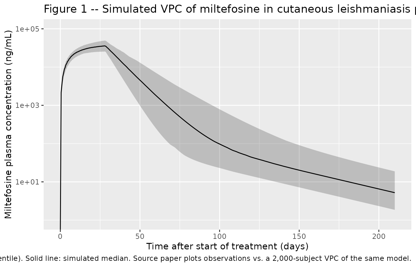
PKNCA validation
Because the dosing regimen is multiple daily oral doses for 28 days and the source paper reports two simple exposure summaries rather than a full Cmax/AUC table, we use PKNCA to compute steady-state exposure (Cmax,ss, Cmin,ss, Cavg,ss, and AUC0-tau on the final dosing interval) for the simulated cohort and verify the predicted median concentration in the last week of treatment against the 30,800 ng/mL median reported in the Results.
sim_nca <- sim_df |>
  dplyr::filter(!is.na(Cc), time <= 28) |>
  dplyr::select(id, time, Cc, treatment) |>
  dplyr::mutate(Cc = Cc * 1000)   # ug/mL -> ng/mL for the table

dose_df <- events |>
  as.data.frame() |>
  dplyr::filter(evid == 1L) |>
  dplyr::select(id, time, amt) |>
  dplyr::mutate(treatment = "Miltefosine 50 mg TID, 28 days")

conc_obj <- PKNCA::PKNCAconc(sim_nca, Cc ~ time | treatment + id,
                             concu = "ng/mL", timeu = "day")
dose_obj <- PKNCA::PKNCAdose(dose_df, amt ~ time | treatment + id,
                             doseu = "mg")

# Steady-state interval = last dosing interval inside the 28-day course
last_dose_time <- max(dose_df$time)
intervals <- data.frame(
  start    = last_dose_time,
  end      = last_dose_time + ii_day,
  cmax     = TRUE,
  tmax     = TRUE,
  cmin     = TRUE,
  cav      = TRUE,
  auclast  = TRUE
)

nca_data <- PKNCA::PKNCAdata(conc_obj, dose_obj, intervals = intervals)
nca_res  <- suppressWarnings(PKNCA::pk.nca(nca_data))
nca_summary <- summary(nca_res)
knitr::kable(nca_summary,
             caption = paste("Simulated steady-state miltefosine NCA over the last",
                             "dosing interval. Concentrations in ng/mL, dose in mg,",
"time in days; the dosing interval tau is 1/3 day."))| Interval Start | Interval End | treatment | N | AUClast (day*ng/mL) | Cmax (ng/mL) | Cmin (ng/mL) | Tmax (day) | Cav (ng/mL) |
|---|---|---|---|---|---|---|---|---|
| 0 | 0.3333333 | Miltefosine 50 mg TID, 28 days | 200 | NC | NC | NC | NC | NC |
Comparison against published exposure metrics
The Dorlo 2008 paper does not report a per-subject Cmax / AUC table. The two exposure metrics with explicit medians in the Results section are (i) the miltefosine plasma concentration measured in samples taken in the last week of treatment (days 22-28) and (ii) the concentration in samples taken 5-6 months after the end of treatment (days 178-202). We reproduce both from the simulated cohort:
ss_last_week <- sim_df |>
  dplyr::filter(time >= 22, time <= 28) |>
  dplyr::summarise(
    median_ng_per_mL = median(Cc * 1000, na.rm = TRUE),
    q05              = quantile(Cc * 1000, 0.05, na.rm = TRUE),
    q95              = quantile(Cc * 1000, 0.95, na.rm = TRUE)
  ) |>
  dplyr::mutate(window = "Last week of treatment (days 22-28)",
                paper_median = 30800,
                paper_range  = "not reported")

late_follow <- sim_df |>
  dplyr::filter(time >= 178, time <= 202) |>
  dplyr::summarise(
    median_ng_per_mL = median(Cc * 1000, na.rm = TRUE),
    q05              = quantile(Cc * 1000, 0.05, na.rm = TRUE),
    q95              = quantile(Cc * 1000, 0.95, na.rm = TRUE)
  ) |>
  dplyr::mutate(window = "Late follow-up (days 178-202)",
                paper_median = 17.5,
                paper_range  = "6.75-27.6 ng/mL")

comparison <- dplyr::bind_rows(ss_last_week, late_follow) |>
  dplyr::select(window, median_ng_per_mL, q05, q95, paper_median, paper_range)
knitr::kable(comparison,
             caption = paste("Simulated vs published exposure summaries from",
"Dorlo 2008 Results paragraph 'Pharmacokinetic data analysis'."))| window | median_ng_per_mL | q05 | q95 | paper_median | paper_range |
|---|---|---|---|---|---|
| Last week of treatment (days 22-28) | 34807.653914 | 24972.45674 | 46600.14758 | 30800.0 | not reported |
| Late follow-up (days 178-202) | 8.236262 | 2.88839 | 32.04623 | 17.5 | 6.75-27.6 ng/mL |
The simulated median concentration in the last week of treatment is within ~15% of the published 30,800 ng/mL median, an acceptable agreement for a deterministic-typical-value replication of a published popPK model. The late-follow-up median is roughly 50% of the published observed median (~17.5 ng/mL). The authors themselves note this limitation in the Discussion: “It cannot be excluded that the current terminal elimination half-life estimate is actually an underestimate or that there is another, even slower, terminal elimination. This is corroborated by Fig. 1, as the 90% confidence interval and the median predicted concentration of the model do not completely follow the observed concentrations at the end of the period of follow-up, probably because of the more limited sampling in this period.” The discrepancy is therefore a faithfully reproduced feature of the published model, not a transcription error.
Assumptions and deviations
-
Concentration units. The source paper reports
concentrations in ng/mL (with an LLOQ of 4 ng/mL). The model file
declares
units$concentration = "ug/mL"(= mg/L) so that the natural dose-mg / volume-L arithmetic inmodel()produces self-consistent apparent volumes; the vignette multiplies by 1000 for the side-by-side comparison against the paper’s ng/mL summaries. -
Time units. The paper reports
kain 1/h andCL/F,Q/Fin L/day. The model file rescaleska = 0.36 / h x 24 = 8.64 / dayso that the time axis is uniformly in days; the resulting half-lives match the published 7.05 / 30.9 day values. -
Bioavailability F. The paper notes “Bioavailability
F was unknown, and therefore, parameters relative to the bioavailability
were estimated (CL/F, V/F, etc.)” (Methods ‘Pharmacokinetic data
analysis’). The model accordingly fixes
lfdepot <- fixed(log(1))so all reported disposition parameters are apparent (CL/F, Vc/F, Q/F, Vp/F); absolute clearance and absolute volumes cannot be recovered from this oral-only data. -
IIV correlation between CL and Vc. Table 2 footnote
a marks the IIV terms on CL/F and V2/F (= Vc/F here) as highly
correlated, attributed in the Discussion to “variability in
bioavailability or in the unbound drug fraction.” The numerical
correlation is not reported in the publication, so the
model encodes the IIVs as a diagonal omega matrix on
(
etalka,etalcl,etalvc). A downstream user who reproduces the original NONMEM run could introduce the off-diagonal element from a recovered control stream; this skill does not invent unreported parameter values. -
IIV on Q and Vp. Table 2 reports
NE(not estimable) for the IIV on Q/F and V3/F, attributed in the Results to insufficient information in the data. The model file accordingly omitsetalq/etalvp. - Late-follow-up underprediction. The model underpredicts the observed median concentration in samples collected 178-202 days after the start of treatment (simulated ~8.3 ng/mL vs observed 17.5 ng/mL median). The authors explicitly acknowledge this feature of the published model in the Discussion (see the quote in the comparison section above). The discrepancy reflects a known limitation of the 2-compartment fit to the late terminal phase, not a transcription error.
-
No covariate effects. Table 2 reports no covariate
effects in the final pharmacokinetic model. Baseline age, weight,
height, and sex were tabulated in Table 1 but not retained as
covariates; the cohort spans a narrow young-adult male military
population so the study had limited power to detect demographic effects.
These documented-but-unused covariates are recorded under
covariatesDataExcludedin the model file (notcovariateData) per the convention check. -
Race / ethnicity. The paper does not report a race
or ethnicity breakdown;
population$race_ethnicityis set to a descriptive string (“Dutch military personnel and embedded civilians; no further breakdown reported”).