BAY81 8973 (Garmann 2017)
Source:vignettes/articles/Garmann_2017_BAY81_8973.Rmd
Garmann_2017_BAY81_8973.RmdModel and source
- Citation: Garmann D, McLeay S, Shah A, Vis P, Maas Enriquez M, Ploeger BA. Population pharmacokinetic characterization of BAY 81-8973, a full-length recombinant factor VIII: lessons learned – importance of including samples with factor VIII levels below the quantitation limit. Haemophilia. 2017 Jul;23(4):528-537. doi:[10.1111/hae.13192](https://doi.org/10.1111/hae.13192)
- Description: Two-compartment population PK model for BAY 81-8973 (Kovaltry, full-length unmodified recombinant human factor VIII) in patients with severe haemophilia A aged 1-61 years pooled from the LEOPOLD I, II, and Kids trials.
- Article: https://doi.org/10.1111/hae.13192
- Modality: Recombinant factor VIII concentrate, IV infusion (typical infusion duration 10 min).
BAY 81-8973 (octocog alfa) is an unmodified full-length recombinant human factor VIII produced in baby hamster kidney cells and intended for replacement therapy in haemophilia A. Garmann 2017 developed a two-compartment population PK model for FVIII activity (chromogenic assay) on data pooled from the three LEOPOLD trials (LEOPOLD I and II in adults / adolescents 12-61 years; LEOPOLD Kids part A in subjects <= 12 years). The chosen final model is fit using the NONMEM M3 likelihood method, which incorporates samples below the lower limit of quantitation (BLQ) rather than excluding them; the central message of the paper is that excluding BLQ samples leads to systematically over-estimated terminal half-lives and therefore under-estimated time spent below a given FVIII threshold. The packaged model uses the final M3 parameter estimates (Table 2 of the paper, identical to the right-hand “final model” column of Table 3).
The structural model is a two-compartment IV model with lean body weight (LBW) as the only covariate, applied as a power function on both clearance and central volume of distribution; the reference LBW is 51.1 kg, the cohort median.
Population
The development cohort comprised 183 male patients with severe haemophilia A pooled from the three LEOPOLD trials (Garmann 2017 Table 1):
- All severe haemophilia A (FVIII activity < 1% by one-stage clotting assay).
- Age 1-61 years (median 22, mean 23.3, SD 14.6).
- Body weight 11-124 kg (median 60, mean 57.7, SD 24.8).
- Height 74-192 cm (median 170, mean 160, SD 25.8).
- BMI 13-38.3 kg/m^2 (median 20.4, mean 21.3, SD 5.14).
- Lean body weight 9.25-79.2 kg (median 51.1, mean 46.2, SD 16.7); used as the covariate-centering reference.
- Race: 132 White, 31 Asian, 10 Black, 9 Hispanic, 1 Other.
- All male (haemophilia A is X-linked).
- Dosing: per-protocol prophylactic IV BAY 81-8973; the analysis included dense PK profiles (10 samples in adults / 4 samples in children following a single infusion) from 43 patients plus pre-dose and 30-min recovery samples from all 183 patients.
- 1535 chromogenic FVIII activity observations were used in the analysis; 16.5% of samples were below the lower limit of quantitation (1.5 IU/dL for the majority; 3 IU/dL for a small number).
The same metadata is available programmatically via
readModelDb("Garmann_2017_BAY81_8973")$population.
Source trace
The per-parameter origin is recorded as an in-file comment next to
each ini() entry in
inst/modeldb/specificDrugs/Garmann_2017_BAY81_8973.R. The
table below collects them in one place for review.
| Parameter (model name) | Value | Source |
|---|---|---|
lcl (typical CL, dL/h) |
log(1.88) | Garmann 2017 Table 2: CL = 1.88 dL/h |
lvc (typical Vc, dL) |
log(30.0) | Garmann 2017 Table 2: Vc = 30.0 dL |
lq (typical CLp, dL/h) |
log(1.90) | Garmann 2017 Table 2: CLp = 1.90 dL/h |
lvp (typical Vp, dL) |
log(6.37) | Garmann 2017 Table 2: Vp = 6.37 dL |
e_lbw_cl (LBW power on CL) |
0.610 | Garmann 2017 Table 2: effect of LBW on CL = 0.610 (95% CI 0.45-0.75) |
e_lbw_vc (LBW power on Vc) |
0.950 | Garmann 2017 Table 2: effect of LBW on Vc = 0.950 (95% CI 0.89-1.02) |
| Reference LBW | 51.1 kg | Garmann 2017 Table 2 footnote: parameterised as
theta * (LBW/51.1)^theta_xx
|
etalcl (omega^2) |
0.12826 | Garmann 2017 Table 2: BSV CL = 37.0% CV; log-normal omega^2 = log(1 + 0.370^2) |
etalvc (omega^2) |
0.01247 | Garmann 2017 Table 2: BSV Vc = 11.2% CV; log-normal omega^2 = log(1 + 0.112^2) |
propSd |
0.267 | Garmann 2017 Table 2: proportional RUV = 26.7% CV |
addSd |
1.10 IU/dL | Garmann 2017 Table 2: additive RUV = 1.10 IU/dL |
Equation: d/dt(central)
|
n/a | Garmann 2017 Methods & Figure 2: two-compartment IV model |
Equation: d/dt(peripheral1)
|
n/a | Garmann 2017 Methods & Figure 2 |
| Combined RUV form | C * (1 + e1) + e2 |
Garmann 2017 Methods, Eq. for C_ij
|
| Reference half-lives | t_half_alpha = 1.85 h, t_half_beta = 13.9 h | Garmann 2017 Table 2 footnote |
The IIV variances above were computed from the reported CV% values
via the log-normal identity omega^2 = log(1 + (CV/100)^2),
consistent with the BSV model P_j = P_pop * exp(eta_j)
stated in Garmann 2017 Methods. Garmann 2017 tested a CL:Vc covariance
during model development but did not retain it (deltaOBJ = 4.8, below
the prespecified retention threshold of 7.9), so etalcl and
etalvc are independent. No IIV was reported on CLp (Q) or
Vp.
Virtual cohort
Original observed FVIII activity data are not publicly available. The
simulations below use a virtual cohort whose demographics approximate
the Garmann 2017 development population, stratified into the four age
bands used in the paper’s PK summary (Table 4): 0 - < 6 years, 6 -
< 12 years, 12 - < 18 years, and >= 18 years. Body weight is
sampled from a log-normal distribution centered on a typical
weight-for-age within each band; lean body weight (LBW) is then derived
from a male-specific approximation of the James (1976) formula:
LBW = 1.10 * WT - 128 * (WT / HT)^2 with WT in kg and HT in
m, capped at the observed Garmann 2017 LBW range (9.25 - 79.2 kg). This
formula is used here purely to populate the covariate column for
simulation; Garmann 2017 itself does not specify the body-composition
formula it used to derive LBW.
set.seed(2017)

james_lbw_male <- function(wt_kg, ht_m) {
  pmin(pmax(1.10 * wt_kg - 128 * (wt_kg / (ht_m * 100))^2, 9.25), 79.2)
}

make_cohort <- function(n, age_min, age_max,
                        wt_log_mean, wt_log_sd, wt_lo, wt_hi,
                        ht_log_mean, ht_log_sd, ht_lo, ht_hi,
                        label, id_offset = 0L) {
  wt <- pmin(pmax(rlnorm(n, log(wt_log_mean), wt_log_sd), wt_lo), wt_hi)
  ht <- pmin(pmax(rlnorm(n, log(ht_log_mean), ht_log_sd), ht_lo), ht_hi)
  tibble(
    ID        = id_offset + seq_len(n),
    AGE       = runif(n, age_min, age_max),
    WT        = wt,
    HT        = ht,
    LBW       = james_lbw_male(wt, ht),
    age_group = label
  )
}

# Per-band sample sizes mirror Garmann 2017 Table 4 (n=24, 27, 23, 109).
cohort <- bind_rows(
  make_cohort( 24, 1,  6,
              wt_log_mean = 16, wt_log_sd = 0.18, wt_lo = 11, wt_hi = 25,
              ht_log_mean = 1.05, ht_log_sd = 0.07, ht_lo = 0.74, ht_hi = 1.20,
              label = "0-<6 y",      id_offset =   0L),
  make_cohort( 27, 6, 12,
              wt_log_mean = 30, wt_log_sd = 0.18, wt_lo = 18, wt_hi = 50,
              ht_log_mean = 1.30, ht_log_sd = 0.05, ht_lo = 1.10, ht_hi = 1.55,
              label = "6-<12 y",     id_offset = 100L),
  make_cohort( 23, 12, 18,
              wt_log_mean = 55, wt_log_sd = 0.18, wt_lo = 35, wt_hi = 90,
              ht_log_mean = 1.65, ht_log_sd = 0.05, ht_lo = 1.45, ht_hi = 1.85,
              label = "12-<18 y",    id_offset = 200L),
  make_cohort(109, 18, 61,
              wt_log_mean = 75, wt_log_sd = 0.20, wt_lo = 50, wt_hi = 124,
              ht_log_mean = 1.75, ht_log_sd = 0.04, ht_lo = 1.55, ht_hi = 1.92,
              label = ">=18 y",      id_offset = 300L)
) |>
  mutate(age_group = factor(age_group,
                            levels = c("0-<6 y", "6-<12 y",
                                       "12-<18 y", ">=18 y")))

stopifnot(!anyDuplicated(cohort$ID))
summary(cohort)
#>        ID             AGE               WT               HT
#>  Min.   :  1.0   Min.   : 1.002   Min.   : 11.25   Min.   :0.9749
#>  1st Qu.:122.5   1st Qu.:10.771   1st Qu.: 35.62   1st Qu.:1.3315
#>  Median :318.0   Median :23.303   Median : 63.06   Median :1.7053
#>  Mean   :256.6   Mean   :26.861   Mean   : 59.24   Mean   :1.5767
#>  3rd Qu.:363.5   3rd Qu.:42.847   3rd Qu.: 77.48   3rd Qu.:1.7668
#>  Max.   :409.0   Max.   :60.377   Max.   :117.80   Max.   :1.9200
#>       LBW           age_group
#>  Min.   :10.76   0-<6 y  : 24
#>  1st Qu.:29.32   6-<12 y : 27
#>  Median :52.10   12-<18 y: 23
#>  Mean   :46.61   >=18 y  :109
#>  3rd Qu.:60.06
#>  Max.   :75.62
A single 50 IU/kg IV bolus dose of BAY 81-8973 is administered at time 0 and FVIII activity is observed over a 96-h window.
obs_grid <- c(0, 0.083, 0.25, 0.5, 1, 2, 4, 6, 8, 12,
              seq(18, 96, by = 6))

build_events <- function(pop) {
  # Garmann 2017 uses LBW; nlmixr2lib's canonical column is LBM (same quantity).
  pop <- pop |> mutate(LBM = LBW)
  amt_per_subject <- pop$WT * 50
  d_dose <- pop |>
    mutate(AMT = amt_per_subject) |>
    tidyr::crossing(TIME = 0) |>
    mutate(EVID = 1, CMT = "central", DV = NA_real_)
  d_obs <- pop |>
    tidyr::crossing(TIME = obs_grid) |>
    mutate(AMT = NA_real_, EVID = 0, CMT = "central", DV = NA_real_)
  bind_rows(d_dose, d_obs) |>
    arrange(ID, TIME, desc(EVID)) |>
    as.data.frame()
}

events <- build_events(cohort)
Simulation
Run a stochastic VPC-style simulation (between-subject variability on CL and Vc included) and a typical-value simulation with the etas zeroed for direct parameter back-checks.
mod <- readModelDb("Garmann_2017_BAY81_8973")

sim <- rxode2::rxSolve(mod, events = events,
                       keep = c("age_group", "WT", "LBM"),
                       returnType = "data.frame")
#> ℹ parameter labels from comments will be replaced by 'label()'
sim <- sim[sim$time >= 0, ]

mod_typ <- rxode2::zeroRe(mod)
#> ℹ parameter labels from comments will be replaced by 'label()'
sim_typ <- rxode2::rxSolve(mod_typ, events = events,
                           keep = c("age_group"),
                           returnType = "data.frame")
#> ℹ omega/sigma items treated as zero: 'etalcl', 'etalvc'
#> Warning: multi-subject simulation without without 'omega'
sim_typ <- sim_typ[sim_typ$time >= 0, ]
FVIII activity-time profiles by age group
Garmann 2017 Figure 5 shows the visual predictive check of the final
model across the development cohort. The figure below reproduces the
typical-value median + 5 - 95% prediction interval of FVIII activity
vs. time after dose, stratified by the four age bands used in the
paper’s per-band PK summary (Table 4). The terminal slope is shallower
in older / heavier patients because LBW power-scaling on Vc (exponent
0.950) is steeper than the LBW power-scaling on CL (exponent 0.610), so
the apparent first-order elimination rate constant of the central
compartment, CL / Vc, scales as
LBW^(0.610 - 0.950) = LBW^(-0.34) and is higher in smaller
patients.
sim_summary <- sim |>
  filter(time > 0) |>
  group_by(time, age_group) |>
  summarise(
    median = stats::median(Cc, na.rm = TRUE),
    lo     = stats::quantile(Cc, 0.05, na.rm = TRUE),
    hi     = stats::quantile(Cc, 0.95, na.rm = TRUE),
    .groups = "drop"
  )

ggplot(sim_summary, aes(time, median, colour = age_group, fill = age_group)) +
  geom_ribbon(aes(ymin = lo, ymax = hi), alpha = 0.18, colour = NA) +
  geom_line(linewidth = 1) +
  scale_y_log10() +
  geom_hline(yintercept = 1.5, linetype = "dashed", colour = "grey40") +
  annotate("text", x = max(obs_grid), y = 1.7,
           label = "LLOQ = 1.5 IU/dL", hjust = 1, vjust = 0,
           colour = "grey30", size = 3) +
  labs(
    x        = "Time after dose (h)",
    y        = "FVIII activity (IU/dL, log scale)",
    colour   = "Age group",
    fill     = "Age group",
    title    = "Simulated BAY 81-8973 PK after a single 50 IU/kg IV dose",
    subtitle = "Stochastic median + 5-95% prediction interval; analogue of Garmann 2017 Figure 5",
    caption  = "Model: Garmann 2017 Haemophilia 23(4):528-537"
  ) +
  theme_bw()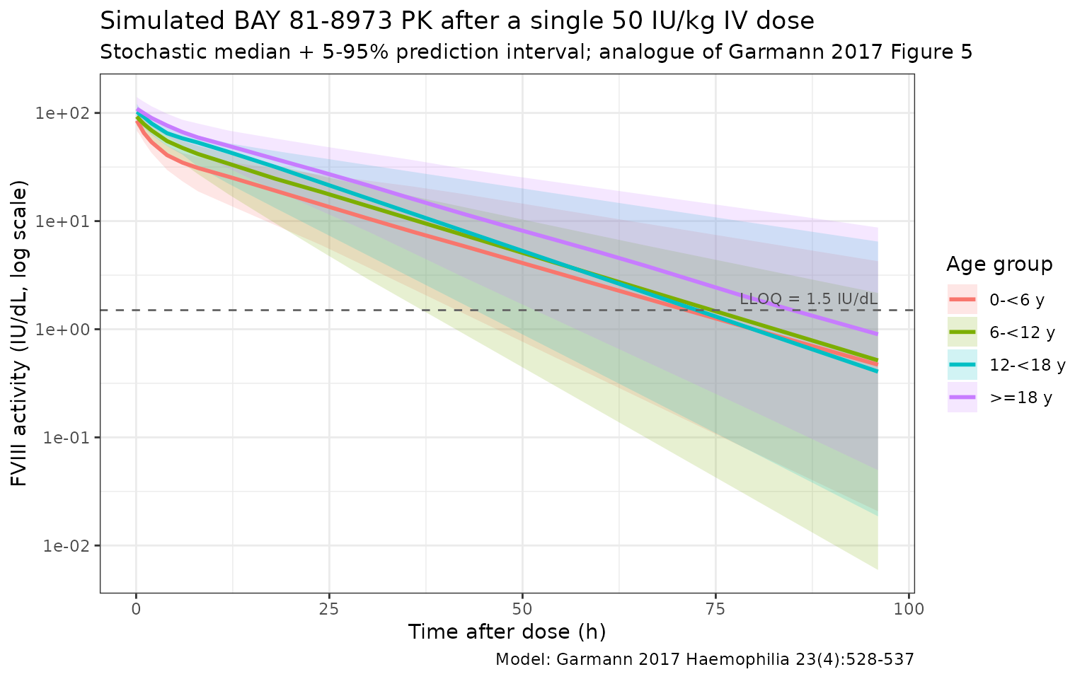
Typical CL and Vss back-check
Garmann 2017 Table 2 reports, for the reference patient (LBW = 51.1 kg), CL = 1.88 dL/h, Vc = 30.0 dL, CLp = 1.90 dL/h, and Vp = 6.37 dL. Table 2 also reports a typical distribution half-life t_half_alpha = 1.85 h and a typical elimination half-life t_half_beta = 13.9 h. Reproducing those numbers from the typical-value simulation is the simplest possible self-consistency check.
ev_ref <- rxode2::et(amt = 50 * 70, time = 0, cmt = "central") |>
  rxode2::et(seq(0, 0))
sim_ref <- rxode2::rxSolve(
  mod_typ, events = ev_ref,
  params = data.frame(LBM = 51.1),
  returnType = "data.frame"
)
#> ℹ omega/sigma items treated as zero: 'etalcl', 'etalvc'

ref_pars <- sim_ref[1, c("cl", "vc", "q", "vp"), drop = FALSE]
ref_pars$Vss <- ref_pars$vc + ref_pars$vp

# Hybrid rate constants and biphasic half-lives derived from CL, Vc, Q, Vp.
kel <- ref_pars$cl / ref_pars$vc
k12 <- ref_pars$q  / ref_pars$vc
k21 <- ref_pars$q  / ref_pars$vp
trace_term <- kel + k12 + k21
disc       <- sqrt(trace_term^2 - 4 * kel * k21)
alpha_h    <- 0.5 * (trace_term + disc)
beta_h     <- 0.5 * (trace_term - disc)
ref_pars$thalf_alpha <- log(2) / alpha_h
ref_pars$thalf_beta  <- log(2) / beta_h

knitr::kable(
  ref_pars,
  caption = "Typical-value PK parameters at the reference 51.1 kg LBW",
  digits  = c(3, 2, 3, 2, 2, 2, 2)
)| cl | vc | q | vp | Vss | thalf_alpha | thalf_beta |
|---|---|---|---|---|---|---|
| 1.88 | 30 | 1.9 | 6.37 | 36.37 | 1.85 | 13.88 |
The model returns CL = 1.88 dL/h, Vc = 30 dL, CLp = 1.9 dL/h, Vp = 6.37 dL, and Vss = Vc + Vp = 36.4 dL with biphasic half-lives t_half_alpha = 1.85 h and t_half_beta = 13.9 h – matching the values reported in Garmann 2017 Table 2 (CL = 1.88 dL/h, Vc = 30.0 dL, CLp = 1.90 dL/h, Vp = 6.37 dL; t_half_alpha = 1.85 h, t_half_beta = 13.9 h).
PKNCA validation
Use PKNCA to compute Cmax, AUC0-inf and terminal half-life by age group, and compare the simulated AUC, weight-normalised CL and weight-normalised Vss against Garmann 2017 Table 4, which reports geometric mean (geometric % CV) PK parameters from empirical Bayes individual estimates after a 50 IU/kg dose.
sim_nca <- sim |>
  filter(!is.na(Cc)) |>
  select(id, time, Cc, age_group)

dose_df <- events |>
  filter(EVID == 1) |>
  transmute(id = ID, time = TIME, amt = AMT, age_group, WT)

conc_obj <- PKNCA::PKNCAconc(sim_nca, Cc ~ time | age_group + id,
                             concu = "IU/dL",
                             timeu = "h")
dose_obj <- PKNCA::PKNCAdose(dose_df, amt ~ time | age_group + id,
                             doseu = "IU")

intervals <- data.frame(
  start      = 0,
  end        = Inf,
  cmax       = TRUE,
  tmax       = TRUE,
  aucinf.obs = TRUE,
  half.life  = TRUE,
  clast.obs  = TRUE,
  lambda.z   = TRUE
)

nca_res <- PKNCA::pk.nca(PKNCA::PKNCAdata(conc_obj, dose_obj,
                                          intervals = intervals))
nca_tbl <- as.data.frame(nca_res$result)

geo_mean    <- function(x) exp(mean(log(x[x > 0]), na.rm = TRUE))
geo_cv_pct  <- function(x) {
  s <- stats::sd(log(x[x > 0]), na.rm = TRUE)
  100 * sqrt(exp(s^2) - 1)
}

auc_summary <- nca_tbl |>
  filter(PPTESTCD == "aucinf.obs") |>
  group_by(age_group) |>
  summarise(
    n             = sum(!is.na(PPORRES)),
    auc_geo_mean  = geo_mean(PPORRES),
    auc_geo_cv    = geo_cv_pct(PPORRES),
    .groups       = "drop"
  )

# Combine with WT and per-subject Vc, Vp from the simulation to derive
# CL/kg = dose/AUC/WT and Vss/kg = (Vc + Vp)/WT for comparison with Table 4.
per_subject <- sim |>
  group_by(id, age_group) |>
  summarise(
    WT  = first(WT),
    LBM = first(LBM),
    Vss = first(vc) + first(vp),
    .groups = "drop"
  )

auc_per_subject <- nca_tbl |>
  filter(PPTESTCD == "aucinf.obs") |>
  transmute(id, age_group, AUC = PPORRES)

combined <- per_subject |>
  left_join(auc_per_subject, by = c("id", "age_group")) |>
  mutate(
    CL_per_kg  = (50 * WT) / AUC / WT,
    Vss_per_kg = Vss / WT
  )

cl_vss_summary <- combined |>
  group_by(age_group) |>
  summarise(
    n              = sum(!is.na(AUC)),
    auc_geo_mean   = geo_mean(AUC),
    auc_geo_cv     = geo_cv_pct(AUC),
    cl_geo_mean    = geo_mean(CL_per_kg),
    cl_geo_cv      = geo_cv_pct(CL_per_kg),
    vss_geo_mean   = geo_mean(Vss_per_kg),
    vss_geo_cv     = geo_cv_pct(Vss_per_kg),
    .groups        = "drop"
  )

knitr::kable(
  cl_vss_summary,
  caption = paste0("Simulated geometric-mean PK parameters by age group ",
                   "after a single 50 IU/kg IV BAY 81-8973 dose."),
  digits  = c(0, 0, 0, 1, 3, 1, 2, 1)
)| age_group | n | auc_geo_mean | auc_geo_cv | cl_geo_mean | cl_geo_cv | vss_geo_mean | vss_geo_cv |
|---|---|---|---|---|---|---|---|
| 0-<6 y | 24 | 1037 | 38.2 | 0.048 | 38.2 | 0.97 | 14.7 |
| 6-<12 y | 27 | 1150 | 38.5 | 0.043 | 38.5 | 0.72 | 13.4 |
| 12-<18 y | 23 | 1627 | 39.4 | 0.031 | 39.4 | 0.60 | 11.5 |
| >=18 y | 109 | 1783 | 40.9 | 0.028 | 40.9 | 0.55 | 13.2 |
Comparison against Garmann 2017 Table 4
Garmann 2017 Table 4 reports geometric mean (geometric % CV) AUC, CL/kg and Vss/kg in four age bands derived from empirical Bayes individual estimates across all LEOPOLD patients. Differences > 20% from the published geometric means would indicate a coding problem.
published <- tibble::tribble(
  ~age_group,       ~published_auc,  ~published_auc_cv,
  ~published_cl,    ~published_cl_cv,
  ~published_vss,   ~published_vss_cv,
  "0-<6 y",         970,    25,    0.05,  25,    0.92,  11,
  "6-<12 y",        1242,   35,    0.04,  35,    0.77,  15,
  "12-<18 y",       1523,   27,    0.03,  27,    0.61,  14,
  ">=18 y",         1858,   38,    0.03,  38,    0.56,  14
) |>
  mutate(age_group = factor(age_group,
                            levels = c("0-<6 y", "6-<12 y",
                                       "12-<18 y", ">=18 y")))

comparison <- published |>
  left_join(cl_vss_summary |>
              select(age_group,
                     simulated_auc = auc_geo_mean,
                     simulated_cl  = cl_geo_mean,
                     simulated_vss = vss_geo_mean),
            by = "age_group") |>
  mutate(
    auc_pct_diff = round(100 * (simulated_auc - published_auc) /
                           published_auc, 1),
    cl_pct_diff  = round(100 * (simulated_cl  - published_cl)  /
                           published_cl, 1),
    vss_pct_diff = round(100 * (simulated_vss - published_vss) /
                           published_vss, 1)
  )

knitr::kable(
  comparison,
  caption = paste0("Simulated vs. Garmann 2017 Table 4 PK parameters ",
                   "by age group at 50 IU/kg dose."),
  digits  = c(0, 0, 3, 0, 2, 0, 0, 3, 2, 1, 1, 1)
)| age_group | published_auc | published_auc_cv | published_cl | published_cl_cv | published_vss | published_vss_cv | simulated_auc | simulated_cl | simulated_vss | auc_pct_diff | cl_pct_diff | vss_pct_diff |
|---|---|---|---|---|---|---|---|---|---|---|---|---|
| 0-<6 y | 970 | 25 | 0 | 25 | 1 | 11 | 1037.436 | 0.05 | 1.0 | 7.0 | -3.6 | 5 |
| 6-<12 y | 1242 | 35 | 0 | 35 | 1 | 15 | 1150.061 | 0.04 | 0.7 | -7.4 | 8.7 | -6 |
| 12-<18 y | 1523 | 27 | 0 | 27 | 1 | 14 | 1627.370 | 0.03 | 0.6 | 6.9 | 2.4 | -2 |
| >=18 y | 1858 | 38 | 0 | 38 | 1 | 14 | 1783.030 | 0.03 | 0.5 | -4.0 | -6.5 | -2 |
Errata
No published erratum was located for Garmann 2017 (Haemophilia 2017;23(4):528-537). The packaged parameter values are taken from Garmann 2017 Table 2 (which is identical to the right-hand “final model” column of Table 3) and the equations stated in the Methods section. The reference LBW of 51.1 kg matches the cohort median LBW reported in Table 1 (51.1 kg, range 9.25-79.2; n = 182).
Assumptions and deviations
-
Lean body weight (LBW) covariate stored as canonical
LBM. Garmann 2017 uses the column nameLBW(lean body weight); the canonical column ininst/references/covariate-columns.mdisLBM(lean body mass). LBW and LBM refer to the same biological quantity (total body weight minus body fat); only the abbreviation differs by literature convention. ThecovariateDataentry in the model file recordssource_name = "LBW". -
LBW body-composition formula not specified. Garmann
2017 does not state the formula used to compute LBW from anthropometric
measurements. In haemophilia popPK literature LBW is most commonly
computed via the Hume
- or James (1976) formula (which give similar results); the
Janmahasatian (2005) FFM formula (the canonical
FFMcolumn) is also sometimes used. The vignette’s virtual cohort uses a male-specific James approximationLBW = 1.10 * WT - 128 * (WT/HT)^2purely to populate the covariate column for simulation; it does not prescribe a specific formula for downstream users.
- or James (1976) formula (which give similar results); the
Janmahasatian (2005) FFM formula (the canonical
-
No CL:Vc covariance in IIV. Garmann 2017 tested a
CL:Vc covariance term during covariate analysis and reported
deltaOBJ = 4.8, below the prespecified 7.9 retention threshold; the covariance was therefore excluded from the final model. The packaged model carries independentetalclandetalvc. - No IIV on CLp (Q) or Vp. Garmann 2017 Table 2 reports BSV only on CL (37.0% CV) and Vc (11.2% CV); no BSV is estimated for the intercompartmental clearance or the peripheral volume.
-
Combined RUV interpreted as
C * (1 + e1) + e2. Garmann 2017 Methods statesC_ij = C_hat * (1 + eps_prop) + eps_add, withpropSdthe SD of the proportional error andaddSdthe SD of the additive error. The packaged model usesCc ~ add(addSd) + prop(propSd), which implements exactly this form in nlmixr2. -
Asian race tested but not retained. Asian race was
the only other significant covariate in the forward selection step
(effect on Vc with
deltaOBJ >= 6.63, P < 0.01), but its removal in backward elimination produced anOBJincrease of 6.68 points (below the 7.9 threshold), so it was not retained. The packaged model has no race covariate, consistent with the published final model. -
Infusion duration handled at the event-table level.
BAY 81-8973 is given as a short IV infusion. Garmann 2017 fixed the
infusion duration to 0.167 h (10 min) where unknown from dosing records.
The packaged model is agnostic to infusion duration; users supply an
RATE(or duration) column in their event table to model the infusion shape if needed. The vignette’s simulations use an instantaneous bolus, which is a reasonable approximation for a 10-min IV infusion when judging trough activity but slightly overestimates very-early Cmax (within ~0.2 h of dose end). -
No baseline FVIII offset. The chromogenic assay
measures total FVIII activity, but in severe haemophilia A baseline
endogenous FVIII activity is by definition < 1 IU/dL (the inclusion
criterion). The packaged model treats simulated
Ccas the activity attributable to BAY 81-8973 above this near-zero baseline; an additive baseline (e.g., 0.5 IU/dL) can be added downstream by the user if desired. - Virtual cohort. Per-band sample sizes (n = 24, 27, 23, 109) match Garmann 2017 Table 4. Body weight and height within each band were simulated from log-normal distributions tuned to span the observed Garmann 2017 Table 1 ranges; LBW was derived from a male James (1976) approximation. Joint covariate structure (e.g., narrow weight range within each pediatric age year, or actual within-trial age-weight correlations) is not simulated.