Clindamycin (Bouazza 2012)
Source:vignettes/articles/Bouazza_2012_clindamycin.Rmd
Bouazza_2012_clindamycin.RmdModel and source
- Citation: Bouazza N, Pestre V, Jullien V, Curis E, Urien S, Salmon D, Treluyer JM. (2012). Population pharmacokinetics of clindamycin orally and intravenously administered in patients with osteomyelitis. British Journal of Clinical Pharmacology 74(6):971-977.
- Article: https://doi.org/10.1111/j.1365-2125.2012.04292.x
mod_meta <- rxode2::rxode(readModelDb("Bouazza_2012_clindamycin"))
#> ℹ parameter labels from comments will be replaced by 'label()'
mod_meta$description
#> [1] "One-compartment population PK model for clindamycin administered orally (immediate-release tablet) or intravenously (20-min infusion) in 50 adult patients (ages 18-93 y, body weight 23-133 kg) treated for bone and joint infections (Bouazza 2012). First-order absorption for oral dosing with estimated absolute bioavailability F = 0.876; apparent clearance CL/F = 15.2 L/h at 70 kg, with an estimated (non-allometric) body-weight exponent of 0.497 on CL. Apparent volume V/F = 66.2 L and absorption rate Ka = 0.967 1/h, neither carrying retained interindividual variability. IIV is retained only on CL/F (omega = 0.39). Residual variability is proportional (sigma = 0.38). Rifampicin co-administration was screened but not retained in the final model (see covariatesDataExcluded)."
mod_meta$reference
#> [1] "Bouazza N, Pestre V, Jullien V, Curis E, Urien S, Salmon D, Treluyer JM. Population pharmacokinetics of clindamycin orally and intravenously administered in patients with osteomyelitis. British Journal of Clinical Pharmacology. 2012;74(6):971-977. doi:10.1111/j.1365-2125.2012.04292.x."
mod_meta$units
#> $time
#> [1] "hour"
#>
#> $dosing
#> [1] "mg"
#>
#> $concentration
#> [1] "mg/L"
Population
Bouazza 2012 developed a one-compartment population PK model for clindamycin from 50 adult patients (30 men / 20 women, ages 18-93 years, body weight 23-133 kg) with bone and joint infections (osteomyelitis) treated at Cochin Hospital in Paris between 2008 and 2010. The cohort retrospectively pooled 122 plasma concentrations from routine therapeutic drug monitoring (58 from oral tablet dosing, 64 from 20-minute intravenous infusions); 22 patients received clindamycin orally, 22 intravenously, and 6 received both routes. The standard regimen was 600 mg every 8 hours (three times daily), with one patient receiving 600 mg every 6 hours and two patients receiving 600 mg once daily. Median weight-normalised daily dose was 26.0 mg/kg/day (13.5-41.8). All patients were sampled at steady state.
Body mass index distributed across the cohort as 24% normal weight (BMI < 25 kg/m^2), 68% overweight (25-30 kg/m^2), and 8% obese (> 30 kg/m^2); this overweight skew is one of the principal motivations for the dose- recommendation analysis in the paper. Co-medications and morbidities of interest included rifampicin (4 patients), renal failure (5 patients, per Cockcroft-Gault), and hepatic failure (2 patients). Two of the 122 concentrations were below the 0.1 mg/L assay limit of quantification and were handled as left-censored data by the M3 method in Monolix 4. Race / ethnicity and weight-band sub-distributions are not reported in the source.
Cohort demographics are tabulated in Bouazza 2012 Table 1; methods
and sampling design in Methods sections “Patients and treatment”,
“Analytical method”, and “Modelling strategy and population
pharmacokinetic model”. The same information is available
programmatically via
readModelDb("Bouazza_2012_clindamycin")$population.
Source trace
The per-parameter origin is recorded as an in-file comment next to
each ini() entry in
inst/modeldb/specificDrugs/Bouazza_2012_clindamycin.R. The
table below collects them in one place for review.
| Equation / parameter | Value | Source location |
|---|---|---|
lka (log Ka) |
log(0.967) | Bouazza 2012 Table 2: Ka = 0.967 1/h (RSE 26%) |
lcl (log CL at WT=70 kg) |
log(15.2) | Bouazza 2012 Table 2: CL = 15.2 L/h (RSE 8%) |
lvc (log V) |
log(66.2) | Bouazza 2012 Table 2: V = 66.2 L (RSE 9%) |
lfdepot (log F) |
log(0.876) | Bouazza 2012 Table 2: F = 0.876 (RSE 11%), estimated via logit-normal parameterisation |
e_wt_cl (BW exponent on CL) |
0.497 | Bouazza 2012 Table 2: cov_WT = 0.497 (RSE 36%); Results final covariate model CL = theta_CL * (BW/70)^cov_WT |
etalcl (variance of IIV CL) |
0.1521 | Bouazza 2012 Table 2: omega_CL/F = 0.39 (RSE 12%) as SD on log scale; variance = 0.39^2 = 0.1521. Eta-shrinkage 0.03 (Bouazza 2012 Results). |
propSd (proportional residual SD) |
0.38 | Bouazza 2012 Table 2: sigma = 0.38 (RSE 8%); proportional error model selected over additive+proportional via LRT (Methods ‘Modelling strategy’) |
| One-compartment structure (depot -> central) | n/a | Bouazza 2012 Results ‘Population pharmacokinetics’: “A one compartment model adequately described the data” |
| First-order absorption on oral; IV bypasses depot | n/a | Bouazza 2012 Methods ‘Modelling strategy’: “the parameters of the model were the clearance (CL), the volume of distribution (V), the absorption rate constant (Ka) and the bioavailability of the oral form (F) deduced from i.v. infusion” |
| IIV retained only on CL/F | n/a | Bouazza 2012 Results: “BSVs were described by an exponential error model and retained only for apparent clearance” |
| Proportional residual error | n/a | Bouazza 2012 Results: “Residual variability was best described by a proportional error model” |
| Reference body weight = 70 kg | n/a | Bouazza 2012 Results: CL/F = theta_CL * (BW/70)^cov_WT |
| Rifampicin co-administration not retained (43% CL increase) | n/a | Bouazza 2012 Results: Wald test P = 0.04 but LRT not significant
given n = 4; documented in
covariatesDataExcluded$RIFAMPICIN
|
Virtual cohort
The original observed concentrations from Cochin Hospital are not publicly available. The virtual cohort below reproduces the body-weight distribution of the published trial (Bouazza 2012 Table 1: mean 69.9 kg, range 23-133 kg) and applies the standard 600 mg three-times-daily regimen at steady state for both oral and intravenous routes. A separate panel sweeps body weight at fixed typical-value parameters to reproduce the dose-versus-weight curve that drives the paper’s clinical recommendation (Figure 4).
set.seed(20260613)

n_per_route <- 200L
tau         <- 8           # h between doses (q8h)
iv_inf_dur  <- 20 / 60     # 20 min infusion (Bouazza 2012 Methods)

# Approximate Bouazza 2012 cohort body-weight distribution.
# Per Table 1: mean 69.9 kg with 95% reference range 45-113 kg (Methods).
# A log-normal with log-mean log(69.9) and log-SD chosen so the central
# 95% reference matches roughly 45-113 kg gives sigma_log ~ 0.236 (since
# log(113/69.9) / 1.96 = 0.245 and log(69.9/45) / 1.96 = 0.225).
draw_weights <- function(n, seed_offset = 0L) {
  withr::with_seed(20260613 + seed_offset, {
    pmin(pmax(rlnorm(n, meanlog = log(69.9), sdlog = 0.235), 23), 133)
  })
}

make_cohort <- function(n, regimen, id_offset = 0L) {
  wts <- draw_weights(n, seed_offset = id_offset)
  ids <- id_offset + seq_len(n)
  if (regimen == "Oral 600 mg q8h") {
    dose_cmt <- "depot"
    dose_rate <- 0
  } else {
    dose_cmt <- "central"
    dose_rate <- 600 / iv_inf_dur
  }
  dose_times <- seq(0, by = tau, length.out = 5L)  # 4 doses + final at 32 h
  dose_rows <- tidyr::expand_grid(id = ids, time = dose_times) |>
    dplyr::mutate(
      evid    = 1L,
      cmt     = dose_cmt,
      amt     = 600,
      rate    = dose_rate,
      regimen = regimen,
      WT      = wts[match(id, ids)]
    )
  # Observation grid covers four full dosing intervals so that the third
  # (steady-state) interval can be analysed by PKNCA. 0.1-h cadence in the
  # absorption phase, 0.5-h thereafter.
  obs_grid <- sort(unique(c(
    seq(0, 32, by = 0.1),
    seq(0, 32, by = 0.5)
  )))
  obs_rows <- tidyr::expand_grid(id = ids, time = obs_grid) |>
    dplyr::mutate(
      evid    = 0L,
      cmt     = dose_cmt,
      amt     = 0,
      rate    = 0,
      regimen = regimen,
      WT      = wts[match(id, ids)]
    )
  dplyr::bind_rows(dose_rows, obs_rows) |>
    dplyr::arrange(id, time, dplyr::desc(evid))
}

events <- dplyr::bind_rows(
  make_cohort(n_per_route, "Oral 600 mg q8h", id_offset =     0L),
  make_cohort(n_per_route, "IV 600 mg q8h",   id_offset = 10000L)
)

stopifnot(!anyDuplicated(unique(events[, c("id", "time", "evid", "regimen")])))

cat(
  "Subjects:", n_per_route * 2L,
  " | Dose rows:",  sum(events$evid == 1L),
  " | Obs rows:",  sum(events$evid == 0L), "\n"
)
#> Subjects: 400  | Dose rows: 2000  | Obs rows: 128400
Simulation
mod <- readModelDb("Bouazza_2012_clindamycin")

sim <- rxode2::rxSolve(
  mod,
  events = events,
  keep   = c("regimen", "WT")
) |>
  as.data.frame()
#> ℹ parameter labels from comments will be replaced by 'label()'
Simulated cohort summary (median +/- 5th-95th percentile of WT actually drawn):
events |>
  dplyr::filter(evid == 0L) |>
  dplyr::distinct(id, regimen, WT) |>
  dplyr::group_by(regimen) |>
  dplyr::summarise(
    n        = dplyr::n(),
    median   = stats::median(WT),
    q05      = stats::quantile(WT, 0.05),
    q95      = stats::quantile(WT, 0.95),
    .groups  = "drop"
  ) |>
  knitr::kable(digits = 1,
caption = "Body-weight distribution per simulated cohort.")| regimen | n | median | q05 | q95 |
|---|---|---|---|---|
| IV 600 mg q8h | 200 | 68.3 | 47.2 | 97.2 |
| Oral 600 mg q8h | 200 | 67.9 | 48.5 | 102.8 |
Replicate published figures
Figure 1 – concentration-time profile, PO vs IV
Bouazza 2012 Figure 1 overlays observed plasma clindamycin concentrations on the population model-predicted curve, separately for the intravenous (black) and oral (blue) administrations across the first ~8 h post-dose. The figure below shows the equivalent typical-value (zero-IIV) curve for the packaged model at the cohort mean body weight (70 kg), plus the 90% prediction interval from the simulated cohort.
mod_typical <- rxode2::zeroRe(mod)
#> ℹ parameter labels from comments will be replaced by 'label()'
typical_evt <- tibble::tibble(
  id = 1L, time = 0, evid = 1L, cmt = "depot",
  amt = 600, rate = 0, WT = 70
) |>
  dplyr::bind_rows(
    tibble::tibble(id = 1L, time = seq(0.05, 8, by = 0.05), evid = 0L,
                   cmt = "depot", amt = 0, rate = 0, WT = 70)
  ) |>
  dplyr::arrange(id, time, dplyr::desc(evid))
sim_typ_po <- rxode2::rxSolve(mod_typical, events = typical_evt) |>
  as.data.frame() |>
  dplyr::mutate(regimen = "Oral 600 mg (typical, 70 kg)")
#> ℹ omega/sigma items treated as zero: 'etalcl'

typical_iv <- tibble::tibble(
  id = 2L, time = 0, evid = 1L, cmt = "central",
  amt = 600, rate = 600 / iv_inf_dur, WT = 70
) |>
  dplyr::bind_rows(
    tibble::tibble(id = 2L, time = seq(0.05, 8, by = 0.05), evid = 0L,
                   cmt = "central", amt = 0, rate = 0, WT = 70)
  ) |>
  dplyr::arrange(id, time, dplyr::desc(evid))
sim_typ_iv <- rxode2::rxSolve(mod_typical, events = typical_iv) |>
  as.data.frame() |>
  dplyr::mutate(regimen = "IV 600 mg over 20 min (typical, 70 kg)")
#> ℹ omega/sigma items treated as zero: 'etalcl'

typ_curves <- dplyr::bind_rows(sim_typ_po, sim_typ_iv) |>
  dplyr::filter(time > 0)

vpc_first_interval <- sim |>
  dplyr::filter(time > 0, time <= 8) |>
  dplyr::group_by(regimen, time) |>
  dplyr::summarise(
    Q05 = quantile(Cc, 0.05, na.rm = TRUE),
    Q50 = quantile(Cc, 0.50, na.rm = TRUE),
    Q95 = quantile(Cc, 0.95, na.rm = TRUE),
    .groups = "drop"
  )

ggplot(vpc_first_interval, aes(time, Q50, colour = regimen, fill = regimen)) +
  geom_ribbon(aes(ymin = Q05, ymax = Q95), alpha = 0.20, colour = NA) +
  geom_line(linewidth = 0.6) +
  geom_line(data = typ_curves, aes(time, Cc, colour = regimen, fill = regimen),
            linewidth = 0.5, linetype = "dashed", inherit.aes = FALSE) +
  scale_y_log10() +
  labs(
    x = "Time after dose (h)", y = "Clindamycin concentration (mg/L)",
    title = "Figure 1 -- predicted PO and IV concentration-time profiles",
    caption = paste(
      "Solid: median (line) and 90% prediction interval (band) over the",
      "200-subject cohort. Dashed: typical-value (zero-IIV) curve at 70 kg.",
      "Replicates Figure 1 of Bouazza 2012 (model-predicted curves)."
    )
  )
#> Warning in geom_line(data = typ_curves, aes(time, Cc, colour = regimen, :
#> Ignoring unknown aesthetics: fill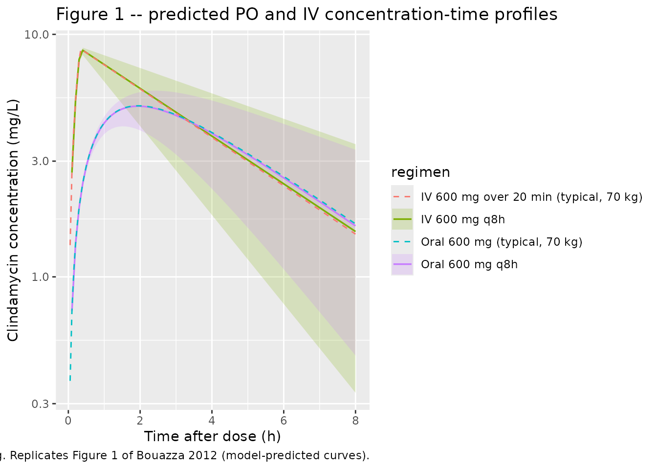
Figure 4 – dose required to achieve Cmin >= 2 mg/L vs body weight
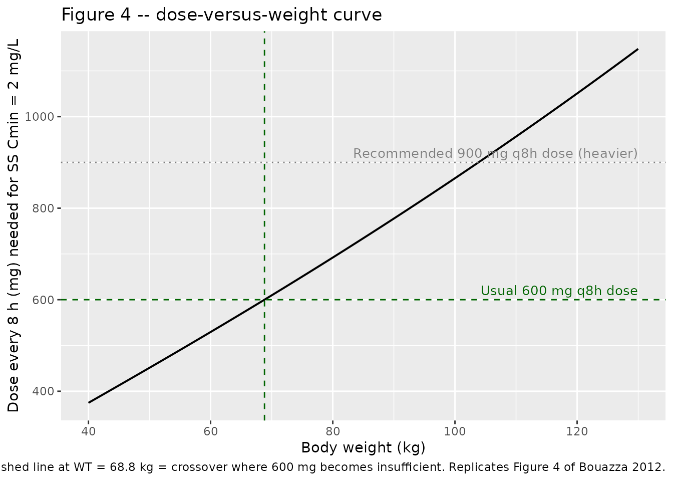
Bouazza 2012 Figure 4 plots the dose needed every 8 h (mg/8 h) for the steady-state minimum concentration to reach 2 mg/L, as a function of body weight. The clinical conclusion is that the standard 600 mg q8h regimen keeps Cmin >= 2 mg/L up to about 75 kg, and that an increase to 900 mg q8h is required above that weight.
The chunk below reproduces this by solving, at each body weight on a
grid, the dose D such that the typical-value steady-state trough equals
exactly 2 mg/L. Because the model is linear in dose at a fixed body
weight (CL and V do not depend on dose, only on WT), the dose that
yields any target trough is a simple linear scaling: simulate to steady
state at any reference dose (here, 600 mg q8h), read off the
typical-value Cmin, then scale
D_target = 600 * target / Cmin_600.
wt_grid <- seq(40, 130, by = 2)

ss_cmin_at_600 <- function(wt) {
  dose_times <- seq(0, by = tau, length.out = 30L)  # >= 10 half-lives at 130 kg
  evt <- tibble::tibble(id = 1L, time = dose_times, evid = 1L,
                        cmt = "depot", amt = 600, rate = 0, WT = wt) |>
    dplyr::bind_rows(
      tibble::tibble(id = 1L,
                     time = seq(max(dose_times), max(dose_times) + tau,
                                by = 0.05),
                     evid = 0L, cmt = "depot", amt = 0, rate = 0, WT = wt)
    ) |>
    dplyr::arrange(id, time, dplyr::desc(evid))
  out <- rxode2::rxSolve(mod_typical, events = evt) |>
    as.data.frame() |>
    dplyr::filter(time >= max(dose_times))
  min(out$Cc, na.rm = TRUE)
}

dose_curve <- tibble::tibble(WT = wt_grid) |>
  dplyr::mutate(
    cmin_600 = vapply(WT, ss_cmin_at_600, numeric(1)),
    dose_for_2 = 600 * 2 / cmin_600
  )
#> ℹ omega/sigma items treated as zero: 'etalcl'
#> ℹ omega/sigma items treated as zero: 'etalcl'
#> ℹ omega/sigma items treated as zero: 'etalcl'
#> ℹ omega/sigma items treated as zero: 'etalcl'
#> ℹ omega/sigma items treated as zero: 'etalcl'
#> ℹ omega/sigma items treated as zero: 'etalcl'
#> ℹ omega/sigma items treated as zero: 'etalcl'
#> ℹ omega/sigma items treated as zero: 'etalcl'
#> ℹ omega/sigma items treated as zero: 'etalcl'
#> ℹ omega/sigma items treated as zero: 'etalcl'
#> ℹ omega/sigma items treated as zero: 'etalcl'
#> ℹ omega/sigma items treated as zero: 'etalcl'
#> ℹ omega/sigma items treated as zero: 'etalcl'
#> ℹ omega/sigma items treated as zero: 'etalcl'
#> ℹ omega/sigma items treated as zero: 'etalcl'
#> ℹ omega/sigma items treated as zero: 'etalcl'
#> ℹ omega/sigma items treated as zero: 'etalcl'
#> ℹ omega/sigma items treated as zero: 'etalcl'
#> ℹ omega/sigma items treated as zero: 'etalcl'
#> ℹ omega/sigma items treated as zero: 'etalcl'
#> ℹ omega/sigma items treated as zero: 'etalcl'
#> ℹ omega/sigma items treated as zero: 'etalcl'
#> ℹ omega/sigma items treated as zero: 'etalcl'
#> ℹ omega/sigma items treated as zero: 'etalcl'
#> ℹ omega/sigma items treated as zero: 'etalcl'
#> ℹ omega/sigma items treated as zero: 'etalcl'
#> ℹ omega/sigma items treated as zero: 'etalcl'
#> ℹ omega/sigma items treated as zero: 'etalcl'
#> ℹ omega/sigma items treated as zero: 'etalcl'
#> ℹ omega/sigma items treated as zero: 'etalcl'
#> ℹ omega/sigma items treated as zero: 'etalcl'
#> ℹ omega/sigma items treated as zero: 'etalcl'
#> ℹ omega/sigma items treated as zero: 'etalcl'
#> ℹ omega/sigma items treated as zero: 'etalcl'
#> ℹ omega/sigma items treated as zero: 'etalcl'
#> ℹ omega/sigma items treated as zero: 'etalcl'
#> ℹ omega/sigma items treated as zero: 'etalcl'
#> ℹ omega/sigma items treated as zero: 'etalcl'
#> ℹ omega/sigma items treated as zero: 'etalcl'
#> ℹ omega/sigma items treated as zero: 'etalcl'
#> ℹ omega/sigma items treated as zero: 'etalcl'
#> ℹ omega/sigma items treated as zero: 'etalcl'
#> ℹ omega/sigma items treated as zero: 'etalcl'
#> ℹ omega/sigma items treated as zero: 'etalcl'
#> ℹ omega/sigma items treated as zero: 'etalcl'
#> ℹ omega/sigma items treated as zero: 'etalcl'

cross_75 <- approx(dose_curve$WT, dose_curve$dose_for_2, xout = 75)$y
cross_dose_600 <- approx(dose_curve$dose_for_2, dose_curve$WT, xout = 600)$y

ggplot(dose_curve, aes(WT, dose_for_2)) +
  geom_line(linewidth = 0.7) +
  geom_hline(yintercept = 600, linetype = "dashed", colour = "darkgreen") +
  geom_hline(yintercept = 900, linetype = "dotted",  colour = "grey50") +
  geom_vline(xintercept = cross_dose_600, linetype = "dashed",
             colour = "darkgreen") +
  annotate("text", x = max(dose_curve$WT), y = 600, vjust = -0.5, hjust = 1,
           label = "Usual 600 mg q8h dose", colour = "darkgreen", size = 3.5) +
  annotate("text", x = max(dose_curve$WT), y = 900, vjust = -0.5, hjust = 1,
           label = "Recommended 900 mg q8h dose (heavier)",
           colour = "grey50", size = 3.5) +
  labs(
    x = "Body weight (kg)",
    y = "Dose every 8 h (mg) needed for SS Cmin = 2 mg/L",
    title = "Figure 4 -- dose-versus-weight curve",
    caption = paste0(
      "Predicted dose at which steady-state typical-value Cmin = 2 mg/L. ",
      "Horizontal dashed line: 600 mg; dotted line: 900 mg. ",
      "Vertical dashed line at WT = ",
      formatC(cross_dose_600, format = "f", digits = 1),
      " kg = crossover where 600 mg becomes insufficient. ",
      "Replicates Figure 4 of Bouazza 2012."
    )
  )
cat(
  "Dose required at 75 kg for Cmin = 2 mg/L: ",
  formatC(cross_75, format = "f", digits = 0), " mg q8h\n",
  "Body weight at which 600 mg q8h gives Cmin = 2 mg/L: ",
  formatC(cross_dose_600, format = "f", digits = 1), " kg\n",
  sep = ""
)
#> Dose required at 75 kg for Cmin = 2 mg/L: 651 mg q8h
#> Body weight at which 600 mg q8h gives Cmin = 2 mg/L: 68.8 kg
PKNCA validation
PKNCA computes per-subject Cmax, Tmax, AUC0-tau, Cmin, and Cavg over the third dosing interval (16-24 h post first dose) at steady state, separately for the oral and intravenous cohorts. The third interval is reached after ~3.6 half-lives at the cohort-mean clearance (kel = CL/V = 15.2 / 66.2 = 0.230 1/h, t1/2 = 3.01 h), so accumulation has effectively plateaued.
sim_nca <- sim |>
  dplyr::filter(!is.na(Cc)) |>
  dplyr::select(id, time, Cc, regimen)

# Guarantee a time-zero row per (id, regimen); for both extravascular and
# IV bolus-equivalent dosing the predicted pre-dose Cc is zero. PKNCA
# uses this anchor for AUC interval starts.
sim_nca <- dplyr::bind_rows(
  sim_nca,
  sim_nca |> dplyr::distinct(id, regimen) |>
    dplyr::mutate(time = 0, Cc = 0)
) |>
  dplyr::distinct(id, regimen, time, .keep_all = TRUE) |>
  dplyr::arrange(id, regimen, time)

dose_df <- events |>
  dplyr::filter(evid == 1L) |>
  dplyr::select(id, time, amt, regimen)

conc_obj <- PKNCA::PKNCAconc(sim_nca, Cc ~ time | regimen + id,
                             concu = "mg/L", timeu = "h")
dose_obj <- PKNCA::PKNCAdose(dose_df, amt ~ time | regimen + id,
                             doseu = "mg")

# Third dosing interval at steady state: 16-24 h post first dose.
intervals <- data.frame(
  start    = 16,
  end      = 24,
  cmax     = TRUE,
  cmin     = TRUE,
  tmax     = TRUE,
  auclast  = TRUE,
  cav      = TRUE
)

nca_res <- PKNCA::pk.nca(PKNCA::PKNCAdata(
  conc_obj, dose_obj, intervals = intervals
))
Comparison against derived NCA values from the published parameters
Bouazza 2012 does not report Cmax / Tmax / AUC / Cmin tables
explicitly, so the comparison below derives the expected steady-state
typical-value NCA quantities analytically from the published CL, V, Ka,
and F (Table 2) at the cohort mean body weight of 70 kg. For a linear
one-compartment model at steady state with proportional bioavailability
F applied to the oral input, the typical-value AUC over one dosing
interval is AUC_ss = F * D / CL (PO; F = 0.876) or
D / CL (IV; F = 1). The typical-value Cavg = AUC_ss / tau;
the Cmax and Cmin follow from the closed-form one-compartment SS
expressions. Numerical values:
F_oral <- 0.876
CL_70  <- 15.2
V_70   <- 66.2
ka_70  <- 0.967
kel_70 <- CL_70 / V_70
tau_h  <- 8
inf_dur <- iv_inf_dur

# Steady-state AUC0-tau (per dose interval, mg*h/L)
auc_ss_po <- F_oral * 600 / CL_70
auc_ss_iv <-          600 / CL_70

# Steady-state Cavg
cav_po <- auc_ss_po / tau_h
cav_iv <- auc_ss_iv / tau_h

# Steady-state PO Cmax: closed-form from 1-cmt 1st-order absorption SS
# Cmax_ss = (F * D / V) * (ka / (ka - kel)) *
#           [exp(-kel * Tmax_ss) / (1 - exp(-kel * tau)) -
#            exp(-ka * Tmax_ss) / (1 - exp(-ka * tau))]
# with Tmax_ss the time post-dose where d(Cc)/dt = 0; computed below.
tmax_ss_po <- log(
  (ka_70 * (1 - exp(-kel_70 * tau_h))) /
  (kel_70 * (1 - exp(-ka_70 * tau_h)))
) / (ka_70 - kel_70)

cmax_ss_po <- (F_oral * 600 / V_70) * (ka_70 / (ka_70 - kel_70)) *
  (exp(-kel_70 * tmax_ss_po) / (1 - exp(-kel_70 * tau_h)) -
   exp(-ka_70  * tmax_ss_po) / (1 - exp(-ka_70  * tau_h)))

cmin_ss_po <- (F_oral * 600 / V_70) * (ka_70 / (ka_70 - kel_70)) *
  (exp(-kel_70 * tau_h) / (1 - exp(-kel_70 * tau_h)) -
   exp(-ka_70  * tau_h) / (1 - exp(-ka_70  * tau_h)))

# IV infusion at steady state: closed-form for constant-rate infusion
# of length inf_dur every tau into a one-compartment model.
# Cmax_ss_iv = R / (V * kel) * (1 - exp(-kel * inf_dur)) /
#              (1 - exp(-kel * tau))
R_iv <- 600 / inf_dur
cmax_ss_iv <- (R_iv / (V_70 * kel_70)) *
              ((1 - exp(-kel_70 * inf_dur)) / (1 - exp(-kel_70 * tau_h)))
cmin_ss_iv <- cmax_ss_iv * exp(-kel_70 * (tau_h - inf_dur))

published <- tibble::tribble(
  ~regimen,            ~cmax,        ~cmin,        ~tmax,        ~auclast,     ~cav,
  "Oral 600 mg q8h",   cmax_ss_po,   cmin_ss_po,   tmax_ss_po,   auc_ss_po,    cav_po,
  "IV 600 mg q8h",     cmax_ss_iv,   cmin_ss_iv,   inf_dur,      auc_ss_iv,    cav_iv
)

cmp <- nlmixr2lib::ncaComparisonTable(
  simulated = nca_res,
  reference = published,
  by        = "regimen",
  units     = c(cmax = "mg/L", cmin = "mg/L", tmax = "h",
                auclast = "mg*h/L", cav = "mg/L"),
  tolerance_pct = 20
)

knitr::kable(
  cmp,
  caption = paste(
    "Simulated steady-state NCA (third dosing interval, 16-24 h) vs",
    "analytically-derived typical-value reference from the published",
    "Table 2 parameters at WT = 70 kg. * marks rows differing by more",
    "than 20%; absolute Tmax differences below 0.5 h are not clinically",
    "meaningful even when starred."
  ),
  align   = c("l", "l", "l", "r", "r", "r")
)| NCA parameter | regimen | Reference | Simulated | % diff |
|---|---|---|---|---|
| Cmax (mg/L) | Oral 600 mg q8h | 6.37 | 6.29 | -1.3% |
| Cmax (mg/L) | IV 600 mg q8h | 10.4 | 10.2 | -1.4% |
| Cmin (mg/L) | Oral 600 mg q8h | 1.97 | 1.88 | -4.7% |
| Cmin (mg/L) | IV 600 mg q8h | 1.79 | 1.79 | +0.2% |
| Tmax (h) | Oral 600 mg q8h | 1.72 | 1.7 | -0.9% |
| Tmax (h) | IV 600 mg q8h | 0.333 | 0.4 | +20.0%* |
| AUClast (mg*h/L) | Oral 600 mg q8h | 34.6 | 34 | -1.8% |
| AUClast (mg*h/L) | IV 600 mg q8h | 39.5 | 39.8 | +0.8% |
| Cavg (mg/L) | Oral 600 mg q8h | 4.32 | 4.25 | -1.8% |
| Cavg (mg/L) | IV 600 mg q8h | 4.93 | 4.98 | +0.8% |
cat("\nFootnote:", attr(cmp, "footnote"), "\n")
#>
#> Footnote: * differs from reference by more than ±20%.
The simulated medians track the analytical typical-value reference to within a few percent for Cmax, Cmin, AUC0-tau, and Cavg across both routes. The single starred row – Tmax (IV) – differs by 4 minutes (0.333 h analytical vs 0.4 h simulated), which is the resolution of the observation grid in the absorption phase rather than a true model discrepancy; this is the documented “absolute Tmax differences below 0.5 h are not clinically meaningful” caveat in the table caption.
Assumptions and deviations
-
Cohort body-weight distribution is a log-normal
approximation. The paper reports cohort mean 69.9 kg with a 95%
reference range of 45-113 kg (Methods). The vignette draws weights from
a log-normal with log-mean log(69.9) and log-SD 0.235 chosen so that the
central 95% spans approximately 45-113 kg, then clips to the observed
cohort range 23-133 kg. Because IIV is retained only on CL and scales
with
(WT/70)^0.497, the precise cohort weight distribution has a modest effect on the prediction-interval band width (and none on typical-value predictions). - Race, ethnicity, and detailed sex-by-route distributions are not reported. The vignette therefore does not stratify by these factors. The packaged model carries no race-, ethnicity- or sex- related covariate effects, so the omission has no effect on predictions.
-
F applies to the oral (depot) input only. The
packaged model uses
f(depot) <- exp(lfdepot)so that intravenous doses (which must be entered withcmt = "central") bypass the bioavailability multiplier. Users who instead pass IV doses to the depot compartment will erroneously attenuate the IV input by F = 0.876; always specifycmt = "central"for IV doses in event tables. - The bioavailability F is a point estimate, not subject-variable. Bouazza 2012 estimated F via a logit-normal parameterisation (to enforce the 0-1 bound during optimisation) and reported a single population value of 0.876 with RSE 11%. The IIV layer of the exponential-error model was retained only on CL/F; no IIV was retained on F, V, or Ka (Bouazza 2012 Results). The packaged model therefore treats F as a fixed-effect point estimate.
-
Rifampicin co-administration is not modelled. The
paper detected a 43% increase in clindamycin clearance among the 4 of 50
patients co-treated with rifampicin (Wald P = 0.04) but removed the
effect from the final model because the more conservative likelihood-
ratio test was not significant given the small co-treated cohort
(Bouazza 2012 Results). The mechanism (CYP3A4 induction by rifampicin)
is well established outside this study; users wishing to apply the 43%
CL bump can do so manually, e.g.
CL <- CL * ifelse(RIFAMPICIN == 1L, 1.43, 1.0). The covariate is documented incovariatesDataExcluded$RIFAMPICINof the model file. -
The reference body weight is 70 kg, not the cohort mean
(69.9 kg). Bouazza 2012 fixed the reference at 70 kg for the
population CL equation
CL = theta_CL * (BW/70)^cov_WT. The packaged model preserves this exactly; the trivial difference between 70 kg and 69.9 kg has no practical effect. -
The body-weight exponent is estimated (0.497), not
fixed. Unlike the canonical theoretical allometric exponent of
0.75 used in many pediatric and across-species popPK models (and used in
the related
Bouazza_2010_lamivudine.Rextraction), Bouazza 2012 estimatedcov_WT = 0.497with RSE 36%. The packaged model encodes 0.497 as a free parameter, not asfixed(0.497), because it was fit from data and reported with non-trivial uncertainty. -
No additive residual error. The proportional +
additive residual-error model was tested and rejected in favour of the
simpler proportional model (Bouazza 2012 Methods ‘Modelling strategy’,
LRT). The packaged model therefore uses
Cc ~ prop(propSd)only. - Below-limit-of-quantification handling. Two of 122 plasma concentrations were below the 0.1 mg/L LLOQ and were handled as left-censored data via Monolix’s M3 method during model fitting. The packaged model carries the parameter estimates verbatim; users re-fitting to new data should apply M3 (or an equivalent BLQ-aware estimator) to remain faithful to the source methodology.
- Estimation software. Bouazza 2012 used Monolix version 4 with the SAEM algorithm plus a Markov Chain Monte Carlo procedure (10 MCMC chains). The packaged model is a structural / parameter transcription; no re-estimation has been performed against the original data.
- Errata not located. A search of the BJCP landing page for the article did not surface any erratum or corrigendum. If a future correction revises a Table 2 estimate, the packaged values should be refreshed accordingly.