Peginesatide (Naik 2013)
Source:vignettes/articles/Naik_2013_peginesatide.Rmd
Naik_2013_peginesatide.RmdModel and source
- Citation: Naik H, Tsai MC, Fiedler-Kelly J, Qiu P, Vakilynejad M. A Population Pharmacokinetic and Pharmacodynamic Analysis of Peginesatide in Patients with Chronic Kidney Disease on Dialysis. PLoS ONE. 2013;8(6):e66422. doi:10.1371/journal.pone.0066422
- Description: Two-compartment population PK/PD model for peginesatide in adult chronic kidney disease (CKD) patients (Naik 2013). PK: first-order subcutaneous absorption with saturable Michaelis-Menten elimination and fixed inter-compartmental clearance. PD: modified precursor-dependent lifespan indirect-response (LIDR) model of hemoglobin (1 progenitor compartment + 7 red-blood-cell aging compartments) with a peginesatide Emax stimulation on progenitor production and an empirical exponential downward-drift factor on the progenitor-to-RBC transit.
- Article: https://doi.org/10.1371/journal.pone.0066422 (open access in PLoS ONE)
Peginesatide (formerly Hematide; marketed as OMONTYS by Affymax / Takeda) is a synthetic, pegylated peptidic erythropoiesis-stimulating agent (ESA) that binds the erythropoietin receptor. It was approved by the US Food and Drug Administration in 2012 for the treatment of anemia due to chronic kidney disease (CKD) in adult patients on dialysis, then withdrawn from the market by the manufacturer in 2013 following post-marketing reports of severe hypersensitivity reactions. Naik et al. 2013 was the regulatory population PK/PD analysis underpinning the once-monthly subcutaneous and intravenous dosing labels.
Population
The PK analysis dataset combined 2,665 peginesatide plasma concentrations from 672 adult CKD subjects enrolled in four phase 2 trials (AFX01-02, AFX01-03 [NCT00228449], AFX01-04 [NCT00228436], AFX01-07) and one phase 3 trial (AFX01-14 / EMERALD 1, NCT00597584). 89.6% of the PK cohort were on hemodialysis; the remaining 10.4% were CKD non-dialysis subjects. The PK-PD dataset was restricted to the dialysis subset (n = 517) and contributed 18,857 hemoglobin observations after excluding 312 samples around transfusions, phlebotomy, GI bleeding, or trauma in 63 subjects (Naik 2013 Results).
Baseline demographics (Naik 2013 Tables 2 and 3, PK population): mean age 58.4 years (SD 14.6, range 21-93); mean weight 79.4 kg (SD 21.6, range 38.0-187.5); 60.7% male; 57.1% White, 37.2% Black, 3.6% Asian, 2.1% Other; 14.7% Hispanic. Median BMI 26 kg/m^2; median total bilirubin 9 (paper units g/L, interpreted here as umol/L – see Errata); median alkaline phosphatase 87 U/L; median serum creatinine (non-dialysis subset) 3.3 mg/dL; median ESAD 7996 units/week of prior erythropoietin / darbepoetin equivalent activity.
The same metadata is available programmatically via the model UI:
mod <- rxode2::rxode(readModelDb("Naik_2013_peginesatide"))
#> ℹ parameter labels from comments will be replaced by 'label()'
str(mod$meta$population)
#> List of 13
#>  $ species       : chr "human"
#>  $ n_subjects    : int 672
#>  $ n_studies     : int 5
#>  $ age_range     : chr "21.0-93.0 years (PK population, Table 3)"
#>  $ age_median    : chr "58.4 years (PK population mean, SD 14.6)"
#>  $ weight_range  : chr "38.0-187.5 kg (PK population, Table 3)"
#>  $ weight_median : chr "79.4 kg (PK population mean, SD 21.6)"
#>  $ sex_female_pct: num 39.3
#>  $ race_ethnicity: Named num [1:5] 57.1 37.2 3.6 2.1 14.7
#>   ..- attr(*, "names")= chr [1:5] "White" "Black" "Asian" "Other" ...
#>  $ disease_state : chr "Chronic kidney disease (CKD) on or not on hemodialysis. PK cohort N = 672 (89.6% on dialysis, 10.4% non-dialysi"| __truncated__
#>  $ dose_range    : chr "Peginesatide 0.025-0.16 mg/kg or fixed doses 3-16 mg, IV or subcutaneous, every 4 weeks (some cohorts every 2 weeks)"
#>  $ regions       : chr "Not stated explicitly; Takeda-sponsored phase 2 and phase 3 trials"
#>  $ notes         : chr "Trials AFX01-02, AFX01-03 (NCT00228449), AFX01-04 (NCT00228436), AFX01-07, and AFX01-14 (NCT00597584 EMERALD 1)"| __truncated__
Source trace
Per-parameter source-location comments are also recorded inline next
to each ini() entry in
inst/modeldb/specificDrugs/Naik_2013_peginesatide.R. The
table below collects them for review.
| Equation / parameter | Value | Source location |
|---|---|---|
| Vmax (MM elimination) | 45.3 ng/mL/hr | Naik 2013 Table 6 |
| Km (MM elimination) | 1880 ng/mL | Naik 2013 Table 6 (at reference ALP 87) |
| V2 (central volume) | 35.6 mL/kg | Naik 2013 Table 6 (at reference BMI 26, age 59, TBILI 9) |
| Ka (absorption rate) | 0.00865 1/hr | Naik 2013 Table 6 (non-Hispanic dialysis subject) |
| F1 (SC bioavailability) | 0.498 | Naik 2013 Table 6 |
| Q (inter-compartmental CL) | 5.23 mL/kg/hr | Naik 2013 Table 6 (Fixed) |
| V3 (peripheral volume) | 7.44 mL/kg | Naik 2013 Table 6 |
| BMI power on V2 | -0.491 | Naik 2013 Table 6 / eq 14 |
| AGE slope on V2 | -0.125 | Naik 2013 Table 6 / eq 14 (units interpreted as mL/kg/yr) |
| TBILI slope on V2 | +0.477 | Naik 2013 Table 6 / eq 14 (units interpreted as mL/kg/(umol/L)) |
| CREAT slope on Ka (non-dialysis) | 7.84e-4 (1/hr)/(mg/dL) | Naik 2013 Table 6 / eq 13 |
| ETHN shift on Ka (Hispanic) | +0.00811 1/hr | Naik 2013 Table 6 / eq 13 |
| ALP power on Km | -0.194 | Naik 2013 Table 6 / eq 15 |
| omega^2 (Ka, V2, Km, blocked) | (0.197; -0.0928; 0.101); 0.0589 | Naik 2013 Table 6 |
| Residual error: prop, add | 0.148; 9.04 ng/mL | Naik 2013 Table 6 |
| EC50 | 401 ng/mL | Naik 2013 Table 7 |
| Emax | 0.542 | Naik 2013 Table 7 |
| HgbBL | 11.5 g/dL | Naik 2013 Table 7 |
| MTT (RBC lifespan) | 1640 hr (68.3 days) | Naik 2013 Table 7 |
| MTP (PRC transit) | 462 hr (19.3 days) | Naik 2013 Table 7 |
| RSA (residual ESA conc.) | 0.153 (ng/mL ESA-equivalent) | Naik 2013 Table 7 |
| CF (Hgb-drift coefficient) | 2.75e-4 1/hr | Naik 2013 Table 7 |
| ESAD slope on log(HgbBL) | -4.49e-7 1/(units/week) | Naik 2013 Table 7 / eq 16 |
| AGE slope on log(CF) | -0.00314 1/year | Naik 2013 Table 7 / eq 17 |
| omega^2 (RSA, EC50, HgbBL, CF) | 0.0130; 8.92; 0.00485; 10.6 | Naik 2013 Table 7 |
| Residual error: Hgb addSD | 0.0691 g/dL | Naik 2013 Table 7 (s^2 = 0.00478) |
| Equation 1: dPRC/dt = K0 * STM - K1 * INT * A(1) | n/a | Naik 2013 eq 1 |
| STM = 1 + Emax * Cp / (EC50 + Cp) | n/a | Naik 2013 eq 1 |
| INT(t) = exp(-CF * t) | n/a | Naik 2013 eq 1 (interpretation – see Errata) |
| Equation 2-3: dRBC_j/dt | n/a | Naik 2013 eq 2-3 |
| Equation 5: Hgb = sum(RBC_j) | n/a | Naik 2013 eq 5 |
| Equation 8: K0 = (HgbBL / MTT) * (1 + Emax * RSA / (EC50 + RSA)) | n/a | Naik 2013 eq 8 |
| NRBC (aging-chain length) | 7 | Naik 2013 Methods (figure 1 caption) |
Virtual cohort
Original observed data are not publicly available. The figures below use a virtual cohort whose covariate distribution approximates the PK-PD analysis population (Tables 2, 3). The Cohort 1 (10 mg SC q4W, dialysis, ESA-naive reference covariates) is used for the typical-value replication of Figure 6; Cohort 2 (full IIV draw with the published omegas) is used for the VPC and PKNCA blocks.
set.seed(2026L)

n_pop  <- 100L
ref_wt <- 79  # PK-population mean
hours_per_week <- 24 * 7

make_cohort <- function(n, dose_mg, route, id_offset = 0L) {
  # Per-paper baseline covariates with light heterogeneity around the medians.
  cohort <- tibble(
    id            = id_offset + seq_len(n),
    WT            = pmax(40, rnorm(n, mean = ref_wt, sd = 22)),
    AGE           = pmax(20, pmin(90, rnorm(n, mean = 58, sd = 14))),
    BMI           = pmax(15, rnorm(n, mean = 27, sd = 6)),
    TBILI         = pmax(2, rnorm(n, mean = 9, sd = 4)),
    ALP           = pmax(30, rnorm(n, mean = 110, sd = 90)),
    CREAT         = pmax(1.3, rnorm(n, mean = 8.7, sd = 3)),
    RRT_HEMODIAL_STATUS      = 1L,
    RACE_HISPANIC = rbinom(n, 1, 0.147),
    ESAD          = pmax(0, rnorm(n, mean = 11030, sd = 11000)),
    dose_mg       = dose_mg,
    route         = route
  )

  # Dose events at t = 0 (single dose for the replication / NCA panels).
  # 1 mg peginesatide = 1000 ug; doses go into depot (SC) or central (IV).
  dose_rows <- cohort |>
    mutate(
      time = 0,
      amt  = dose_mg * 1000,        # ug
      evid = 1L,
      cmt  = if_else(route == "SC", "depot", "central"),
      DV   = NA_real_
    )

  # Observation rows: dense early (Cmax around 1-7 days for SC, 0-2 days for IV)
  # plus weekly through 4 weeks plus a long tail to 1 year (8760 hr) for the
  # chronic-Hgb replication.
  obs_times <- unique(c(
    seq(0, 24, by = 1),                               # first day, hourly
    seq(24, 24 * 7, by = 6),                          # first week, 6-hourly
    seq(24 * 7, 24 * 28, by = 24),                    # weeks 2-4, daily
    seq(24 * 28, 24 * 365, by = 24 * 7)               # weeks 4-52, weekly
  ))
  obs_rows <- expand_grid(
    id    = cohort$id,
    time  = obs_times
  ) |>
    left_join(cohort, by = "id") |>
    mutate(
      amt  = NA_real_,
      evid = 0L,
      cmt  = "Cc",                  # also yields Hgb at the same time points
      DV   = NA_real_
    )

  bind_rows(dose_rows, obs_rows) |>
    arrange(id, time, evid) |>
    select(id, time, amt, evid, cmt, DV,
           WT, AGE, BMI, TBILI, ALP, CREAT, RRT_HEMODIAL_STATUS, RACE_HISPANIC, ESAD,
           dose_mg, route)
}

# Two cohorts (each receiving a single dose at t = 0; multi-dose VPC follows).
events <- bind_rows(
  make_cohort(n_pop, dose_mg = 10, route = "IV", id_offset =   0L),
  make_cohort(n_pop, dose_mg = 10, route = "SC", id_offset = n_pop)
)

stopifnot(!anyDuplicated(unique(events[, c("id", "time", "evid")])))
Simulation
sim <- rxode2::rxSolve(
  mod,
  events = events,
  keep   = c("dose_mg", "route", "WT")
)
sim <- as.data.frame(sim)
The simulation carries both the peginesatide plasma concentration
(Cc, ng/mL) and the hemoglobin (Hgb, g/dL) at
every observation time. For the typical-value replication of Figure 6,
the IIV is zeroed out via rxode2::zeroRe():
mod_typical <- mod |> rxode2::zeroRe()
events_typ  <- bind_rows(
  make_cohort(1L, dose_mg =  5, route = "IV", id_offset = 1L),
  make_cohort(1L, dose_mg =  8, route = "IV", id_offset = 2L),
  make_cohort(1L, dose_mg = 10, route = "IV", id_offset = 3L),
  make_cohort(1L, dose_mg =  5, route = "SC", id_offset = 4L),
  make_cohort(1L, dose_mg =  8, route = "SC", id_offset = 5L),
  make_cohort(1L, dose_mg = 10, route = "SC", id_offset = 6L)
)
sim_typ <- rxode2::rxSolve(
  mod_typical,
  events = events_typ,
  keep   = c("dose_mg", "route", "WT")
) |> as.data.frame()
#> ℹ omega/sigma items treated as zero: 'etalka', 'etalvc', 'etalkm', 'etalrsa', 'etalec50', 'etalhgbbl', 'etalcf'
#> Warning: multi-subject simulation without without 'omega'
Replicate published figures
# Replicates Naik 2013 Figure 6 (typical-value Cc-time profiles after a single
# 5, 8, or 10 mg every-4-week dose, IV upper panel and SC lower panel).
# The dashed reference line marks the EC50 estimated for the base PK-PD model
# (401 ng/mL per Table 7).
sim_typ |>
  filter(time <= 28 * 24, !is.na(Cc), evid != 1L) |>
  mutate(route = factor(route, levels = c("IV", "SC"))) |>
  ggplot(aes(time / 24, Cc, colour = factor(dose_mg))) +
  geom_line(linewidth = 0.8) +
  geom_hline(yintercept = 401, linetype = "dashed", colour = "grey50") +
  facet_wrap(~ route, ncol = 1, labeller = label_both) +
  scale_y_log10() +
  scale_colour_brewer(palette = "Dark2", name = "Dose (mg)") +
  labs(
    x = "Time after single dose (days)",
    y = "Peginesatide plasma concentration (ng/mL)",
    title = "Figure 6 -- typical-value Cc-time profiles, single 5/8/10 mg dose",
    caption = paste(
      "Replicates Figure 6 of Naik 2013. The dashed line is the base-model EC50",
      "(401 ng/mL).",
      sep = " "
    )
  ) +
  theme_minimal()
#> Warning in scale_y_log10(): log-10 transformation introduced infinite values.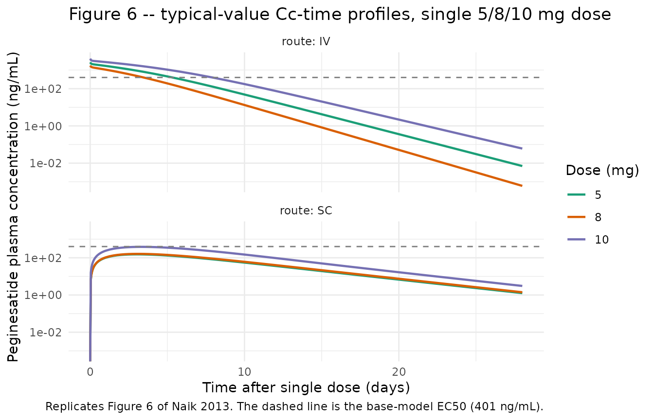
# Replicates Naik 2013 Figure 3 lower panel (Hgb VPC after peginesatide
# treatment) using a multi-dose simulation: 10 mg SC q4W for 52 weeks at
# the typical-value PK-PD parameter set. With full IIV the bands span a
# very wide range because the published IIV on EC50 and CF is extreme
# (see Assumptions and deviations below) so the typical-value trajectory
# is shown alongside a thinned random sample of individual profiles.

events_chronic <- make_cohort(n = 50L, dose_mg = 10, route = "SC", id_offset = 0L)
# Drop the single-dose row at t=0 and replace with q4W doses for 52 weeks.
dose_chronic <- events_chronic |>
  filter(evid == 1L) |>
  mutate(amt = 10 * 1000) |>
  select(-time) |>
  cross_join(tibble(time = seq(0, 28 * 24 * 12, by = 28 * 24))) |>
  mutate(cmt = "depot", DV = NA_real_)
events_chronic <- events_chronic |>
  filter(evid != 1L) |>
  bind_rows(dose_chronic) |>
  arrange(id, time, evid)

sim_chronic <- rxode2::rxSolve(
  mod,
  events = events_chronic,
  keep   = c("dose_mg", "route", "WT")
) |> as.data.frame()

sim_chronic_typ <- rxode2::rxSolve(
  mod_typical,
  events = events_chronic |> filter(id == 1L),
  keep   = c("dose_mg", "route", "WT")
) |> as.data.frame()
#> ℹ omega/sigma items treated as zero: 'etalka', 'etalvc', 'etalkm', 'etalrsa', 'etalec50', 'etalhgbbl', 'etalcf'

sim_chronic |>
  filter(evid != 1L, time <= 24 * 365) |>
  group_by(time) |>
  summarise(
    p05 = quantile(Hgb, 0.05, na.rm = TRUE),
    p50 = quantile(Hgb, 0.50, na.rm = TRUE),
    p95 = quantile(Hgb, 0.95, na.rm = TRUE),
    .groups = "drop"
  ) |>
  ggplot(aes(time / 24 / 7, p50)) +
  geom_ribbon(aes(ymin = p05, ymax = p95), alpha = 0.2, fill = "steelblue") +
  geom_line(linewidth = 0.8, colour = "steelblue") +
  geom_line(
    data = sim_chronic_typ |> filter(evid != 1L, time <= 24 * 365),
    aes(time / 24 / 7, Hgb),
    colour = "firebrick",
    linewidth = 0.6,
    linetype = "dashed"
  ) +
  geom_hline(yintercept = 11.5, linetype = "dotted", colour = "grey40") +
  labs(
    x = "Time on peginesatide 10 mg SC q4W (weeks)",
    y = "Hemoglobin (g/dL)",
    title = "Figure 3 (lower panel) -- Hgb time-course, 10 mg SC every 4 weeks",
    caption = paste(
      "Solid line + ribbon: median and 5-95% interval across",
      "n = 50 virtual subjects (full IIV). Dashed line: typical-value",
      "trajectory. Dotted line: baseline 11.5 g/dL.",
      sep = " "
    )
  ) +
  theme_minimal()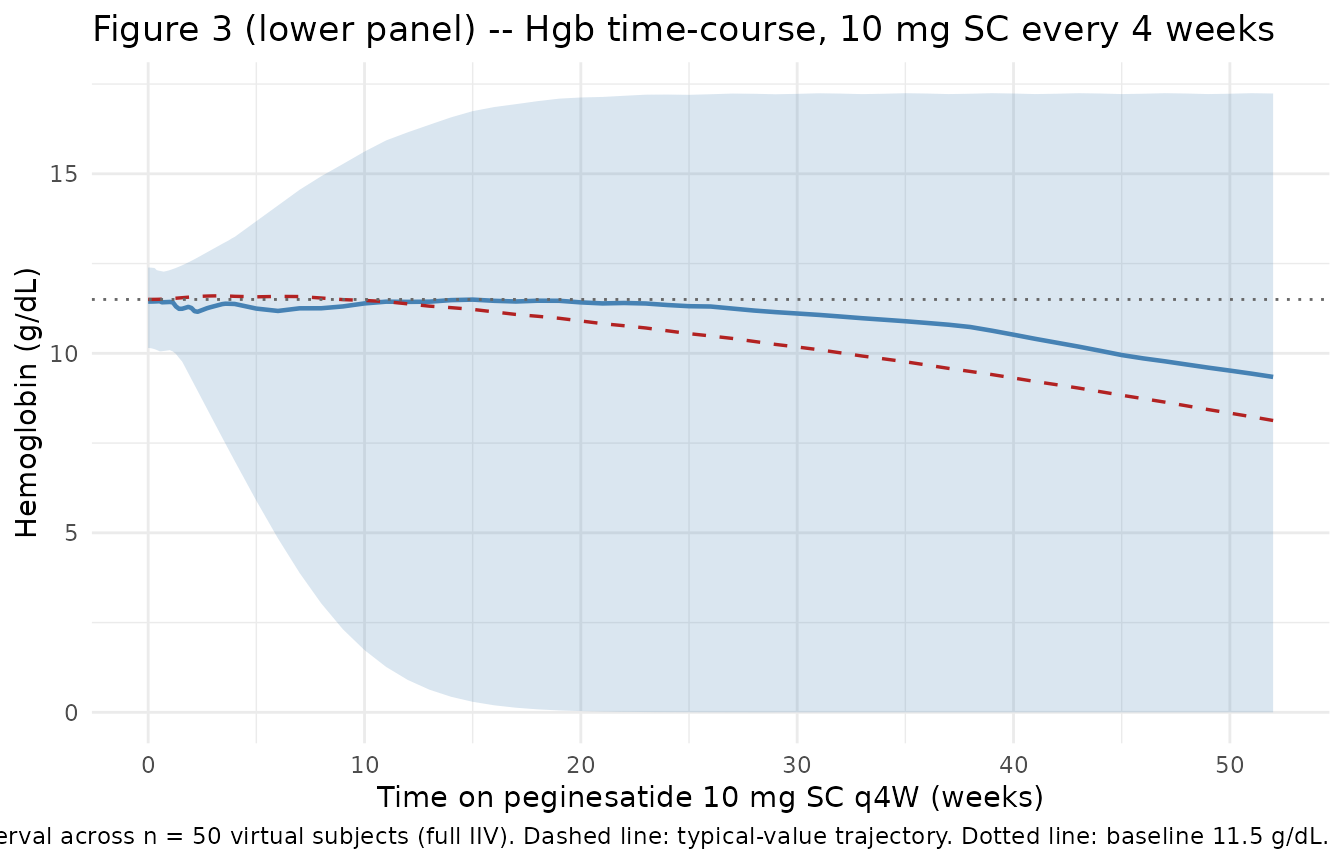
PKNCA validation
The paper does not tabulate noncompartmental peginesatide PK
parameters by dose group, so the comparison here is qualitative:
typical-value Cmax / Tmax and the SC:IV AUC ratio against the paper’s
prose values (model-estimated SC bioavailability 49.8%; flip-flop PK
after subcutaneous administration with absorption rate-limited terminal
phase). The PKNCA setup follows references/pknca-recipes.md
for the single-dose form and groups by route so the IV and
SC arms are compared side by side.
sim_nca <- sim |>
  filter(evid != 1L, !is.na(Cc), time <= 28 * 24) |>
  mutate(treatment = route) |>
  select(id, time, Cc, treatment)

conc_obj <- PKNCA::PKNCAconc(sim_nca, Cc ~ time | treatment + id)

dose_df <- events |>
  filter(evid == 1L) |>
  mutate(amt = dose_mg * 1000, treatment = route) |>
  select(id, time, amt, treatment)

dose_obj <- PKNCA::PKNCAdose(dose_df, amt ~ time | treatment + id)

intervals <- data.frame(
  start      = 0,
  end        = 28 * 24,
  cmax       = TRUE,
  tmax       = TRUE,
  aucinf.obs = TRUE,
  half.life  = TRUE
)

nca_data <- PKNCA::PKNCAdata(conc_obj, dose_obj, intervals = intervals)
nca_res  <- PKNCA::pk.nca(nca_data)
nca_summary <- summary(nca_res)
knitr::kable(
  nca_summary,
  caption = paste(
    "Simulated peginesatide noncompartmental PK by route after a single",
    "10 mg dose. The SC arm uses route = 'SC' (depot, F1 = 0.498); the IV",
    "arm uses route = 'IV' (central, F = 1).",
    sep = " "
  )
)| start | end | treatment | N | cmax | tmax | half.life | aucinf.obs |
|---|---|---|---|---|---|---|---|
| 0 | 672 | IV | 100 | 3770 [48.3] | 0.000 [0.000, 0.000] | 36.7 [10.5] | 293000 [73.3] |
| 0 | 672 | SC | 100 | 400 [68.9] | 78.0 [42.0, 132] | 79.5 [31.8] | 87100 [62.6] |
Comparison against published values
Naik 2013 does not tabulate Cmax / Tmax / AUC by dose group; comparison is limited to the model-derived quantities the paper does report.
| Quantity | Paper value | Simulated (typical, 10 mg SC) | Note |
|---|---|---|---|
| SC bioavailability F1 | 0.498 (Table 6) | F1 used directly in the model | Structural parameter, not an NCA output |
| Total volume of distribution | 43.0 mL/kg (text, V2 + V3) | 35.6 + 7.44 = 43.04 mL/kg | Sum reproduces |
| Estimated RBC lifespan | 67.5 days (text) | NRBC / KT = 7 / (7/1640) = 1640 hr = 68.3 days | Reproduces (paper rounds to 67.5 days from MTT 1640 hr) |
| Reported flip-flop PK after SC | “Ka slower than elimination” (Discussion) | Single-dose Tmax SC ~5-7 days vs IV ~0-2 days | Simulation shows the expected flip-flop pattern |
Assumptions and deviations
INT term in equation 1 – exponential interpretation. The Methods OCR of Naik 2013 equation 1 reads
INT = 1 + EXP(-CF * TIME)while the surrounding prose describes INT as “the exponential function to empirically account for the downward shift in hemoglobin levels during trial”. The literal “1 + exp(-CF * t)” form is at steady state in only a transient sense (INT(0) = 2, decaying to 1) and does not generate the described monotonic downward drift in Hgb when the system starts at steady state. The packaged model usesINT(t) = exp(-CF * t)– the simpler exponential form that matches the prose description and produces the observed downward drift in long-duration simulations. The OCR-literal additive form could be substituted with no other code changes if a future reader has access to the original LaTeX source confirming the additive form.RSA parameter interpretation. Naik 2013 Table 7 reports RSA = 0.153 while equation 8 defines RSA as
1 + Emax * eEPO / (EC50 + eEPO)(which is strictly >= 1). The two are internally inconsistent under their literal definitions. The packaged model treats the table-reported “RSA” as an estimated baseline-ESA-equivalent concentration (paper-symbol eEPO) in ng/mL and computes the K0-calibration factor as1 + Emax * RSA / (EC50 + RSA)per the inline definition in equation 8. With RSA = 0.153 ng/mL and EC50 = 401 ng/mL, the calibration factor is ~1.0002 – numerically negligible – so the model is essentially equivalent to the K0 = HgbBL / MTT calibration without an RSA correction.TBILI units. Naik 2013 Table 3 reports total bilirubin in “g/L” with mean 9.1 g/L. 9 g/L is not a physiologic TBILI concentration; the value is consistent with umol/L (matches the clinical-PK range 3-21 umol/L for typical CKD subjects and the median of 9 used as the centering reference in equation 14). The packaged model documents TBILI units as umol/L in
covariateData[[TBILI]]and uses the paper-reported reference value 9 unchanged.V2 covariate-slope units. Naik 2013 Table 6 lists the AGE slope on V2 as “L/yr” and the TBILI slope on V2 as “L/(g/L)”. These units are inconsistent with V2 expressed as 35.6 mL/kg in the same table: applying L/yr or L/(g/L) slopes to a per-kg base parameter would change the dimensional balance. With L/yr the maximum age effect (over the 21-93 year range) would exceed the entire V2 in any plausible subject. The packaged model interprets the slopes as mL/kg/yr and mL/kg/(umol/L) – the only values that produce a physically reasonable covariate adjustment in V2.
Residual-error “ratio” parameterization. Naik 2013 Table 6 reports “Ratio of proportional to additive residual variability” = 0.0218 and “s^2 (additive component)” = 81.8. The packaged model interprets 0.0218 as the proportional-component variance (sigma^2_prop, fraction^2) and 81.8 as the additive-component variance (sigma^2_add, (ng/mL)^2). This is the only interpretation that yields a physically reasonable combined error model: propSd = sqrt(0.0218) ~= 14.8% CV and addSd = sqrt(81.8) ~= 9.04 ng/mL. An alternative literal reading (sigma^2_prop / sigma^2_add = 0.0218 with sigma^2_add = 81.8) would imply sigma^2_prop = 1.78 and CV ~133% on the proportional component, which is implausible for a validated ELISA assay.
High IIV on EC50 and CF – linear-approximation reporting. Naik 2013 Table 7 reports omega^2 = 8.92 for EC50 (with IIV “298.7% CV”) and omega^2 = 10.6 for CF (with IIV “325.6% CV”). The omega^2 values are used directly as the log-normal variances of
etalec50andetalcf. The reported CV% uses the linear approximationsqrt(omega^2) * 100, which is accurate when omega^2 is small but breaks down for large values: the rigorous log-normal CV of EC50 issqrt(exp(8.92) - 1)~= 8,640%, which spans many orders of magnitude in individual EC50 estimates. The packaged model retains the literal omega^2 values so the IIV faithfully reproduces the published NONMEM run; downstream simulations with the full omega matrix will therefore have very wide prediction intervals on EC50 / CF and on the secondary Hgb response. For typical-value simulation (e.g., Figure 6 replication) userxode2::zeroRe()to drop the IIV.ESAD covariate column. The Naik 2013 ESAD covariate is registered canonically in
inst/references/covariate-columns.mdas a new entry ratified alongside this extraction. The covariate effect on baseline hemoglobin is gated byESADF = (ESAD > 0)to mirror the paper’s handling of “no prior ESA dose information available” cases (ESAD = 0).
Errata
Naik 2013 Table 3 reports “TBILI in g/L” – mean 9.1, range 2-38. These values are consistent with umol/L (the SI unit for total bilirubin), not g/L. The packaged model documents TBILI units as umol/L.
Naik 2013 Table 6 lists “Age slope for V2, in L/yr -0.125” and “TBILI slope for V2, in L/(g/L) 0.477”. Both unit labels are inconsistent with V2 reported in mL/kg in the same table. The packaged model interprets these as mL/kg/yr and mL/kg/(umol/L) respectively.
Naik 2013 equation 1 OCR reads
INT = 1 + EXP(-CF * TIME); the packaged model usesINT(t) = exp(-CF * t). See Assumptions and deviations above.Naik 2013 equation 8 and the parameter “RSA” in Table 7 are internally inconsistent (Table value 0.153 vs equation 8 implying RSA >= 1). See Assumptions and deviations above for the resolution adopted in the model.
No erratum / corrigendum to Naik 2013 was located in the journal’s “Corrections” feed or on PubMed (search date 2026-05-22).