Tacrolimus (Agergaard 2025)
Source:vignettes/articles/Agergaard_2025_tacrolimus.Rmd
Agergaard_2025_tacrolimus.RmdModel and source
- Citation: Agergaard K, Thiesson HC, Carstens J, Staatz CE, Jarvinen E, Nielsen F, Christensen HD, Juhl-Sandberg R, Brosen K, Stage TB, Andersen DT, Kjellsson MC, Bergmann TK. Population pharmacokinetics of tacrolimus whole blood and peripheral blood mononuclear cell concentrations in stable kidney-transplanted patients. Br J Clin Pharmacol. 2025;91(3):761-773. doi:10.1111/bcp.16277
- Description: Two-compartment population PK model for oral immediate-release tacrolimus in stable adult kidney transplant recipients (Agergaard 2025), fitted jointly to whole-blood and peripheral blood mononuclear cell (PBMC) concentrations. First-order absorption (ka = 1/MTT) after a lag time and linear elimination. The PBMC concentration is an algebraic observable, not an ODE state: distribution into PBMCs was found to be instantaneous, so Cpbmc = R_C:PBMC * Cc, where the PBMC:whole-blood ratio carries a Box-Cox-transformed IIV, fractional-shift effects of CYP3A5 non-expressor status and NR1I2 -25385C>T (rs3814055) homozygous-mutant genotype, and a 0.709 dilution multiplier for PBMC samples visibly contaminated with erythrocytes. CYP3A5 non-expressor status lowers CL/F, female sex lowers Vc/F, and relative bioavailability (fixed to 1 at age 59 years, with IIV) increases exponentially with age. Separate proportional residual errors for whole blood and PBMC.
- Article: Br J Clin Pharmacol 2025;91(3):761-773 (open access, PMC11862786)
The paper links whole-blood and intracellular (peripheral blood mononuclear cell, PBMC) tacrolimus concentrations in a single population model. The whole-blood part is a two-compartment model with lagged first-order absorption. Distribution into PBMCs was found to be instantaneous, so the PBMC concentration is an algebraic rescaling of the central concentration (Equation 2):
There is no PBMC compartment and no PBMC rate constant in the final model.
Population
Agergaard 2025 enrolled 63 stable adult kidney transplant recipients (>= 3 months after transplantation; median 38 months, IQR 15-79) at three Danish nephrology departments between June 2021 and October 2023. All took immediate-release tacrolimus twice daily with mycophenolate, at steady state (no dose change in the preceding 5 days); the median tacrolimus dose was 2 mg and a whole-blood trough of 5 ng/mL was generally targeted. Median age was 59 years (IQR 48-68), median weight 86.8 kg, 71.4% were male and 95.2% Caucasian. Eleven patients (17.5%) were CYP3A5 expressers and 11 (17.5%) were homozygous for NR1I2 -25385T (rs3814055). Patients were sampled on one occasion, densely (n = 18; 11 samples over 12 h) or sparsely (n = 45; predose, 0.5, 1.5 and 4 h), giving 366 whole-blood and 348 PBMC concentrations, all measured by LC-MS/MS (Methods 2.1, Results 3.1, Table 1).
The same information is available programmatically:
str(readModelDb("Agergaard_2025_tacrolimus")()$population, give.attr = FALSE)
#> List of 17
#>  $ species                     : chr "human"
#>  $ n_subjects                  : int 63
#>  $ n_studies                   : int 1
#>  $ n_observations              : chr "366 whole-blood and 348 PBMC concentrations"
#>  $ age_range                   : chr "IQR 48-68 years"
#>  $ age_median                  : chr "59 years"
#>  $ weight_range                : chr "IQR 73.4-98.3 kg"
#>  $ weight_median               : chr "86.8 kg"
#>  $ sex_female_pct              : num 28.6
#>  $ race_ethnicity              : Named num [1:2] 95.2 4.8
#>  $ disease_state               : chr "Stable adult kidney transplant recipients (>= 3 months post-transplant; median 38 months, IQR 15-79) on immedia"| __truncated__
#>  $ dose_range                  : chr "Oral immediate-release tacrolimus twice daily; median dose 2 mg (IQR 1.2-2.0 mg as printed in Table 1); whole-b"| __truncated__
#>  $ regions                     : chr "Denmark (Odense, Esbjerg and Kolding nephrology departments), June 2021 - October 2023."
#>  $ cyp3a5_distribution         : chr "11 expressers (17.5%), 52 non-expressers (82.5%) (Table 1)."
#>  $ nr1i2_rs3814055_distribution: chr "CC 31 (49.2%), CT 21 (33.3%), TT 11 (17.5%) (Table 1)."
#>  $ sampling                    : chr "One occasion per patient: dense (n = 18; predose and 0.5, 1, 1.5, 2, 3, 4, 6, 8, 10, 12 h) or sparse (n = 45; p"| __truncated__
#>  $ notes                       : chr "Agergaard 2025 Methods 2.1, Results 3.1 and Table 1. Tacrolimus measured by LC-MS/MS in both matrices (LOQ 0.20 ng/mL)."
Source trace
Every ini() value carries an in-file comment pointing to
its source. All values are the “Final model with covariates” column of
Table 2. The PDF encodes minus signs as control characters, so the signs
of the CYP3A5-on-CL/F, female and lambda rows were read from the
rendered table and cross-checked against the Discussion’s
percentages.
| Parameter / equation | Value | Source location |
|---|---|---|
lcl (CL/F, CYP3A5 expresser) |
log(28.2) L/h | Table 2, footnote a |
e_cyp3a5_nonexpr_cl |
-0.466 | Table 2; Discussion “46.6% lower CL/F” |
lvc (Vc/F, male) |
log(180) L | Table 2, footnote b |
e_sexf_vc |
-0.345 | Table 2; Discussion “34.5% lower” |
lq (Q/F) |
log(51.0) L/h | Table 2 |
lvp (Vp/F) |
log(1688) L | Table 2 |
lfdepot (F at 59 years) |
fixed(log(1)) | Table 2 footnotes c, d; Results 3.2 |
e_age_fdepot |
0.0123 per year | Table 2; form from Figure 4A (see below) |
lmtt (ka = 1/MTT) |
log(0.676) h | Table 2; Results 3.2; Figure 2 |
ltlag |
log(0.369) h | Table 2 |
lratio_pbmc_central (R_C:PBMC) |
log(1.96) | Table 2, footnote f; Equation 2 |
e_cyp3a5_nonexpr_ratio_pbmc_central |
0.424 | Table 2; Discussion “42.4% higher” |
e_nr1i2_hom_ratio_pbmc_central |
0.607 | Table 2; Discussion “60.7% higher” |
e_sample_rbc_contam_ratio_pbmc_central |
0.709 | Table 2; Results 3.2 “70.9% of R_C:PBMC without redness” |
boxcox_lratio_pbmc_central (lambda) |
-2.50 | Table 2 |
etalcl |
0.210^2 | Table 2 IIV 21.0% |
etalfdepot |
0.410^2 | Table 2 IIV 41.0% |
etalmtt |
1.29^2 | Table 2 IIV 129% |
etalratio_pbmc_central |
0.378^2 | Table 2 IIV 37.8%; Results 3.2 (Box-Cox) |
propSd |
0.137 | Table 2 RUV_C 13.7% |
propSd_Cpbmc |
0.354 | Table 2 RUV_PBMC 35.4% |
| Two-compartment ODEs, lag, first-order absorption | n/a | Results 3.2; Methods 2.5; Figure 2 |
Cpbmc <- ratio_pbmc_central * Cc |
n/a | Equation 2 |
| Covariate forms (fractional shifts; exponential age) | n/a | Methods 2.6; Table 2; Discussion; Figure 4 |
mod <- readModelDb("Agergaard_2025_tacrolimus")
ui <- rxode2::rxode(mod)
#> ℹ parameter labels from comments will be replaced by 'label()'
# The model must integrate its explicit ODEs, not an auto-detected solved system.
stopifnot(is.null(ui$linCmt) || isFALSE(ui$linCmt))
mod_typ <- rxode2::zeroRe(ui)
Simulation helpers
The study population was at steady state on twice-daily dosing. The
terminal half-life implied by Table 2 is long (Vp/F = 1688 L), so the
helpers below dose for 100 intervals and observe the last one. With two
declared endpoints (Cc and Cpbmc), observation
rows nominate the endpoint with dvid; both concentrations
are returned as columns on every observation row.
tau <- 12
n_dose <- 100
t_last <- (n_dose - 1) * tau
obs_rel <- sort(unique(c(
  0,
  seq(0.30, 3, by = 0.02),
  seq(3.25, tau, by = 0.25)
)))

# One row per subject in `subj` (columns: id plus covariates) -> event table.
make_events <- function(subj, dose_mg = 2) {
  dose <- subj |>
    tidyr::crossing(time = (seq_len(n_dose) - 1) * tau) |>
    mutate(amt = dose_mg, evid = 1L, cmt = "depot", dvid = NA_integer_)
  obs <- subj |>
    tidyr::crossing(time = t_last + obs_rel) |>
    mutate(amt = 0, evid = 0L, cmt = NA_character_, dvid = 1L)
  bind_rows(dose, obs) |>
    arrange(id, time, desc(evid)) |>
    select(id, time, amt, evid, cmt, dvid, everything())
}

ref_subject <- function(id = 1L, ...) {
  base <- tibble(
    id = id, AGE = 59, SEXF = 0, CYP3A5_EXPR = 1,
    SNP_NR1I2_RS3814055_HOM = 0, SAMPLE_RBC_CONTAM = 0
  )
  mods <- list(...)
  for (nm in names(mods)) base[[nm]] <- mods[[nm]]
  base
}

solve_ss <- function(model, subj, omega = NULL) {
  args <- list(
    model, make_events(subj),
    keep = setdiff(names(subj), "id"), returnType = "data.frame"
  )
  if (!is.null(omega)) args$omega <- omega
  out <- withCallingHandlers(
    as.data.frame(do.call(rxode2::rxSolve, args)),
    # Typical-value solves use zeroRe(), for which this warning is expected.
    warning = function(w) {
      if (grepl("without 'omega'", conditionMessage(w), fixed = TRUE)) {
        invokeRestart("muffleWarning")
      }
    }
  )
  if (is.null(out$id)) out$id <- subj$id[1]
  out$tad <- out$time - t_last
  out
}

auc_trap <- function(t, y) sum(diff(t) * (head(y, -1) + tail(y, -1)) / 2)
Deterministic structure checks
Steady-state mass balance
Over a steady-state dosing interval, AUC must equal F * Dose / CL. This checks the dose route, the bioavailability, the mg-to-ng/mL conversion and that the ODEs are integrated as written.
mb <- bind_rows(
  ref_subject(1L),
  ref_subject(2L, CYP3A5_EXPR = 0),
  ref_subject(3L, AGE = 31),
  ref_subject(4L, SEXF = 1)
)
mb_sim <- solve_ss(mod_typ, mb)
#> ℹ omega/sigma items treated as zero: 'etalcl', 'etalfdepot', 'etalmtt', 'etalratio_pbmc_central'
mb_tab <- mb_sim |>
  group_by(id) |>
  summarise(
    AGE = first(AGE), SEXF = first(SEXF), CYP3A5_EXPR = first(CYP3A5_EXPR),
    auc_sim = auc_trap(tad, Cc),
    auc_expected = 1000 * 2 * first(fdepot) / first(cl),
    .groups = "drop"
  ) |>
  mutate(pct_diff = 100 * (auc_sim / auc_expected - 1))
knitr::kable(mb_tab, digits = 3)| id | AGE | SEXF | CYP3A5_EXPR | auc_sim | auc_expected | pct_diff |
|---|---|---|---|---|---|---|
| 1 | 59 | 0 | 1 | 70.930 | 70.922 | 0.012 |
| 2 | 59 | 0 | 0 | 132.775 | 132.813 | -0.028 |
| 3 | 31 | 0 | 1 | 50.265 | 50.259 | 0.012 |
| 4 | 59 | 1 | 1 | 70.935 | 70.922 | 0.019 |
Covariate relationships: Figure 4
Figure 4 overlays the typical-individual prediction (green dashed line) on the individual estimates. The maintainers digitised those lines from the published figure; the packaged model’s typical values reproduce every one to within about 1%.
fig4 <- tibble::tribble(
  ~panel, ~group, ~digitised, ~model,
  "4B Vc/F (L)", "male", 180.6, 180,
  "4B Vc/F (L)", "female", 118.3, 180 * (1 - 0.345),
  "4C CL/F (L/h)", "CYP3A5 expresser", 28.19, 28.2,
  "4C CL/F (L/h)", "CYP3A5 non-expresser", 15.05, 28.2 * (1 - 0.466),
  "4D R_C:PBMC", "expresser, CC/CT", 1.973, 1.96,
  "4D R_C:PBMC", "expresser, TT", 3.164, 1.96 * 1.607,
  "4D R_C:PBMC", "non-expresser, CC/CT", 2.799, 1.96 * 1.424,
  "4D R_C:PBMC", "non-expresser, TT", 4.507, 1.96 * 1.424 * 1.607
)

# Confirm the "model" column is what the packaged model actually computes.
grid4 <- bind_rows(
  ref_subject(1L), ref_subject(2L, SEXF = 1),
  ref_subject(3L, CYP3A5_EXPR = 0),
  ref_subject(4L, SNP_NR1I2_RS3814055_HOM = 1),
  ref_subject(5L, CYP3A5_EXPR = 0, SNP_NR1I2_RS3814055_HOM = 1)
)
s4 <- solve_ss(mod_typ, grid4) |>
  group_by(id) |>
  summarise(vc = first(vc), cl = first(cl), R = first(Cpbmc / Cc), .groups = "drop")
#> ℹ omega/sigma items treated as zero: 'etalcl', 'etalfdepot', 'etalmtt', 'etalratio_pbmc_central'
stopifnot(
  isTRUE(all.equal(s4$vc[1:2], fig4$model[1:2])),
  isTRUE(all.equal(s4$cl[c(1, 3)], fig4$model[3:4])),
  isTRUE(all.equal(s4$R[c(1, 4, 3, 5)], fig4$model[5:8]))
)

fig4 <- fig4 |> mutate(pct_diff = 100 * (model / digitised - 1))
fig4 |>
  dplyr::rename(
    "Figure panel" = panel, "Group" = group, "Digitised" = digitised,
    "Model" = model, "Difference (%)" = pct_diff
  ) |>
knitr::kable(digits = 3)| Figure panel | Group | Digitised | Model | Difference (%) |
|---|---|---|---|---|
| 4B Vc/F (L) | male | 180.600 | 180.000 | -0.332 |
| 4B Vc/F (L) | female | 118.300 | 117.900 | -0.338 |
| 4C CL/F (L/h) | CYP3A5 expresser | 28.190 | 28.200 | 0.035 |
| 4C CL/F (L/h) | CYP3A5 non-expresser | 15.050 | 15.059 | 0.058 |
| 4D R_C:PBMC | expresser, CC/CT | 1.973 | 1.960 | -0.659 |
| 4D R_C:PBMC | expresser, TT | 3.164 | 3.150 | -0.451 |
| 4D R_C:PBMC | non-expresser, CC/CT | 2.799 | 2.791 | -0.284 |
| 4D R_C:PBMC | non-expresser, TT | 4.507 | 4.485 | -0.484 |
Functional form of the age effect on F
Table 2 gives the age coefficient (0.0123) but not the functional form; Methods 2.6 says continuous covariates were normalised to the median and tested as linear, exponential and power functions. The typical-individual line of Figure 4A, digitised below, separates the three readings.
fig4a <- tibble::tribble(
  ~AGE, ~F_digitised,
  21, 0.628,
  31, 0.710,
  59, 1.000,
  75, 1.214,
  81, 1.302
)
age_forms <- fig4a |>
  mutate(
    exponential = exp(0.0123 * (AGE - 59)),
    linear = 1 + 0.0123 * (AGE - 59),
    power = (AGE / 59)^0.0123
  )
knitr::kable(age_forms, digits = 3)| AGE | F_digitised | exponential | linear | power |
|---|---|---|---|---|
| 21 | 0.628 | 0.627 | 0.533 | 0.987 |
| 31 | 0.710 | 0.709 | 0.656 | 0.992 |
| 59 | 1.000 | 1.000 | 1.000 | 1.000 |
| 75 | 1.214 | 1.218 | 1.197 | 1.003 |
| 81 | 1.302 | 1.311 | 1.271 | 1.004 |
rms <- function(x) sqrt(mean(x^2))
age_rms <- c(
  exponential = rms(age_forms$exponential - age_forms$F_digitised),
  linear = rms(age_forms$linear - age_forms$F_digitised),
  power = rms(age_forms$power - age_forms$F_digitised)
)
age_rms
#> exponential      linear       power
#> 0.004302121 0.051657178 0.261587086
stopifnot(
  age_rms[["exponential"]] < 0.01,
  age_rms[["linear"]] > 3 * age_rms[["exponential"]],
  age_rms[["power"]] > 3 * age_rms[["exponential"]]
)

# The packaged model uses the exponential form.
s_age <- solve_ss(mod_typ, tibble(
  id = 1:5, AGE = fig4a$AGE, SEXF = 0, CYP3A5_EXPR = 1,
  SNP_NR1I2_RS3814055_HOM = 0, SAMPLE_RBC_CONTAM = 0
)) |>
  distinct(id, fdepot)
#> ℹ omega/sigma items treated as zero: 'etalcl', 'etalfdepot', 'etalmtt', 'etalratio_pbmc_central'
stopifnot(isTRUE(all.equal(s_age$fdepot, age_forms$exponential)))
The exponential form matches the digitised line almost exactly (a free exponential fit to the line recovers 0.0123 per year with F = 1.000 at 59 years). The linear form is off by about 0.09 at 21 years, and the median-ratio power form is nearly flat.
Covariate profiles: Figure 5
Figure 5 shows steady-state whole-blood and PBMC profiles for pairs of covariate values. The paper does not state the dose or the values of the covariates that were held fixed. The profiles below are typical-value predictions at 2 mg twice daily (the Table 1 median dose) for a 59-year-old male CYP3A5 expresser carrying a NR1I2 -25385 C allele unless the panel varies that covariate.
f5_groups <- tibble::tribble(
  ~panel, ~label, ~AGE, ~SEXF, ~CYP3A5_EXPR, ~SNP_NR1I2_RS3814055_HOM,
  "A Sex", "Man", 59, 0, 1, 0,
  "A Sex", "Woman", 59, 1, 1, 0,
  "B Age", "31 years", 31, 0, 1, 0,
  "B Age", "75 years", 75, 0, 1, 0,
  "C NR1I2-25385C>T", "CC or CT", 59, 0, 1, 0,
  "C NR1I2-25385C>T", "TT", 59, 0, 1, 1,
  "D CYP3A5", "Expresser", 59, 0, 1, 0,
  "D CYP3A5", "Non-expresser", 59, 0, 0, 0,
  "E Extremes", "75 y man, TT, non-expresser", 75, 0, 0, 1,
  "E Extremes", "31 y woman, CC/CT, expresser", 31, 1, 1, 0
) |>
  mutate(id = seq_len(n()), SAMPLE_RBC_CONTAM = 0)

f5_sim <- solve_ss(
  mod_typ,
  select(f5_groups, id, AGE, SEXF, CYP3A5_EXPR, SNP_NR1I2_RS3814055_HOM, SAMPLE_RBC_CONTAM)
) |>
  left_join(select(f5_groups, id, panel, label), by = "id")
#> ℹ omega/sigma items treated as zero: 'etalcl', 'etalfdepot', 'etalmtt', 'etalratio_pbmc_central'

f5_sim |>
  select(panel, label, tad, `Whole blood` = Cc, PBMC = Cpbmc) |>
  pivot_longer(c(`Whole blood`, PBMC), names_to = "matrix", values_to = "conc") |>
  mutate(matrix = factor(matrix, c("Whole blood", "PBMC"))) |>
  ggplot(aes(tad, conc, colour = label)) +
  geom_line() +
  facet_grid(panel ~ matrix, scales = "free_y") +
  labs(
    x = "Time after dose (h)", y = "Typical concentration (model units)",
    colour = NULL,
    caption = "Replicates the layout of Figure 5 of Agergaard 2025 (typical values, 2 mg b.i.d.)."
  ) +
  theme_bw() +
  theme(legend.position = "bottom") +
  guides(colour = guide_legend(ncol = 2))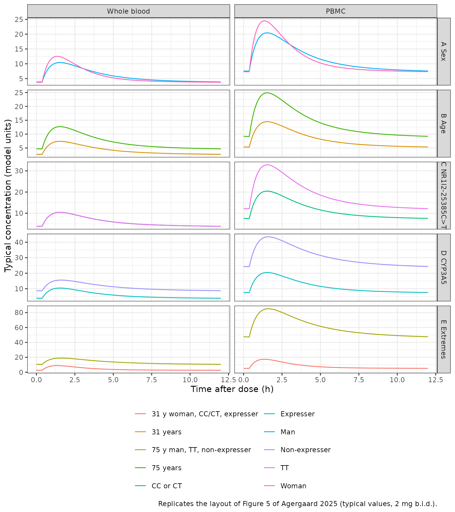
f5_tab <- f5_sim |>
  group_by(panel, label) |>
  summarise(
    auc_wb = auc_trap(tad, Cc),
    cmax_wb = max(Cc),
    ctrough_wb = last(Cc),
    ratio_pbmc = first(Cpbmc / Cc),
    .groups = "drop"
  )
f5_tab |>
  dplyr::rename(
    "Panel" = panel, "Group" = label, "Whole-blood AUC0-12 (ng*h/mL)" = auc_wb,
    "Whole-blood Cmax (ng/mL)" = cmax_wb, "Whole-blood trough (ng/mL)" = ctrough_wb,
    "Cpbmc / Cc" = ratio_pbmc
  ) |>
knitr::kable(digits = 2)| Panel | Group | Whole-blood AUC0-12 (ng*h/mL) | Whole-blood Cmax (ng/mL) | Whole-blood trough (ng/mL) | Cpbmc / Cc |
|---|---|---|---|---|---|
| A Sex | Man | 70.93 | 10.43 | 3.86 | 1.96 |
| A Sex | Woman | 70.94 | 12.50 | 3.73 | 1.96 |
| B Age | 31 years | 50.26 | 7.39 | 2.73 | 1.96 |
| B Age | 75 years | 86.36 | 12.70 | 4.70 | 1.96 |
| C NR1I2-25385C>T | CC or CT | 70.93 | 10.43 | 3.86 | 1.96 |
| C NR1I2-25385C>T | TT | 70.93 | 10.43 | 3.86 | 3.15 |
| D CYP3A5 | Expresser | 70.93 | 10.43 | 3.86 | 1.96 |
| D CYP3A5 | Non-expresser | 132.78 | 15.59 | 8.71 | 2.79 |
| E Extremes | 31 y woman, CC/CT, expresser | 50.27 | 8.86 | 2.65 | 1.96 |
| E Extremes | 75 y man, TT, non-expresser | 161.65 | 18.98 | 10.61 | 4.49 |
f5v <- function(lab, col) f5_tab[[col]][f5_tab$label == lab]
stopifnot(
  # Sex acts on Vc/F only: same exposure, sharper peak in women.
  abs(f5v("Woman", "auc_wb") / f5v("Man", "auc_wb") - 1) < 0.005,
  f5v("Woman", "cmax_wb") > f5v("Man", "cmax_wb"),
  # Age acts on F: exposure scales by exp(0.0123 * 44).
  abs(f5v("75 years", "auc_wb") / f5v("31 years", "auc_wb") / exp(0.0123 * 44) - 1) < 0.005,
  # NR1I2 acts on R only.
  abs(f5v("TT", "auc_wb") / f5v("CC or CT", "auc_wb") - 1) < 0.005,
  abs(f5v("TT", "ratio_pbmc") - 1.96 * 1.607) < 1e-6,
  # CYP3A5 acts on CL/F and R.
  abs(f5v("Non-expresser", "auc_wb") / f5v("Expresser", "auc_wb") - 1 / (1 - 0.466)) < 0.01,
  abs(f5v("Non-expresser", "ratio_pbmc") - 1.96 * 1.424) < 1e-6
)
Three features of Figure 5 are reproduced: the NR1I2 genotype moves only the PBMC profile (panel C); the CYP3A5 non-expresser has about 1.9-fold higher whole-blood exposure and a further 1.42-fold higher PBMC:blood ratio (panel D); and in every panel the plotted PBMC curve sits at R_C:PBMC times the whole-blood curve, with the PBMC axis numerically on the whole-blood scale. Two panels of the published figure cannot be reproduced from Table 2; see “Assumptions and deviations”.
Virtual cohort
The cohort below approximates Table 1. Patient-level data are not
public. Age is drawn from a normal distribution matching the median and
IQR (59, 48-68 years; values outside the 18-85-year eligibility band are
redrawn, not clamped); sex, CYP3A5 status and NR1I2 -25385 TT status are
drawn independently at the Table 1 frequencies. All PBMC samples are
taken as uncontaminated (SAMPLE_RBC_CONTAM = 0). The study
titrated doses to a trough target, so a single 2 mg twice-daily dose for
everyone (the Table 1 median) overstates the spread of exposures
relative to the observed data.
set.seed(20250301)
rxode2::rxSetSeed(20250301)

draw_age <- function(n, median = 59, sd = 20 / 1.349, lo = 18, hi = 85) {
  out <- rnorm(n, median, sd)
  bad <- out < lo | out > hi
  while (any(bad)) {
    out[bad] <- rnorm(sum(bad), median, sd)
    bad <- out < lo | out > hi
  }
  out
}

n_sub <- 200
cohort <- tibble(
  id = seq_len(n_sub),
  AGE = draw_age(n_sub),
  SEXF = rbinom(n_sub, 1, 18 / 63),
  CYP3A5_EXPR = rbinom(n_sub, 1, 11 / 63),
  SNP_NR1I2_RS3814055_HOM = rbinom(n_sub, 1, 11 / 63),
  SAMPLE_RBC_CONTAM = 0
)
summary(cohort[, -1])
#>       AGE             SEXF        CYP3A5_EXPR    SNP_NR1I2_RS3814055_HOM
#>  Min.   :23.50   Min.   :0.000   Min.   :0.000   Min.   :0.000
#>  1st Qu.:49.79   1st Qu.:0.000   1st Qu.:0.000   1st Qu.:0.000
#>  Median :59.32   Median :0.000   Median :0.000   Median :0.000
#>  Mean   :58.50   Mean   :0.275   Mean   :0.175   Mean   :0.285
#>  3rd Qu.:66.55   3rd Qu.:1.000   3rd Qu.:0.000   3rd Qu.:1.000
#>  Max.   :84.59   Max.   :1.000   Max.   :1.000   Max.   :1.000
#>  SAMPLE_RBC_CONTAM
#>  Min.   :0
#>  1st Qu.:0
#>  Median :0
#>  Mean   :0
#>  3rd Qu.:0
#>  Max.   :0
Simulation and comparison with Figure 3
sim <- solve_ss(mod, cohort) |>
  mutate(cyp3a5 = ifelse(CYP3A5_EXPR == 1, "Expresser", "Non-expresser"))
#> ℹ parameter labels from comments will be replaced by 'label()'

vpc <- sim |>
  select(id, tad, `Whole blood (ng/mL)` = Cc, `PBMC (model units)` = Cpbmc) |>
  pivot_longer(-c(id, tad), names_to = "matrix", values_to = "conc") |>
  group_by(matrix, tad) |>
  summarise(
    p10 = quantile(conc, 0.10), p50 = median(conc), p90 = quantile(conc, 0.90),
    .groups = "drop"
  )

ggplot(vpc, aes(tad)) +
  geom_ribbon(aes(ymin = p10, ymax = p90), alpha = 0.25, fill = "seagreen") +
  geom_line(aes(y = p50)) +
  scale_y_log10() +
  facet_wrap(~matrix, scales = "free_y") +
  labs(
    x = "Time after dose (h)", y = "Concentration",
    caption = "Compare with Figure 3A,B of Agergaard 2025 (median and 10th-90th percentiles)."
  ) +
  theme_bw()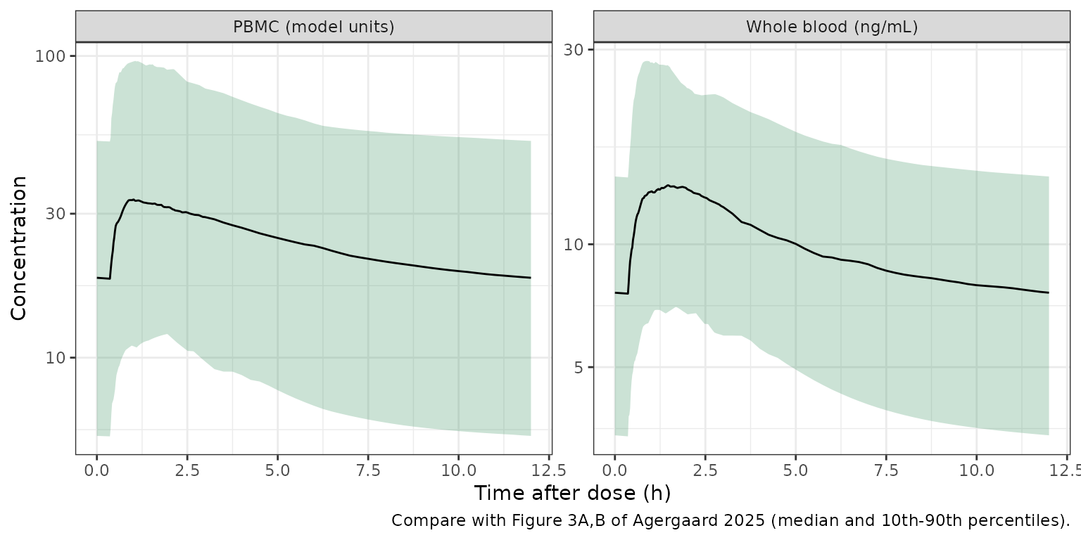
wb_med <- vpc |> filter(matrix == "Whole blood (ng/mL)")
wb_trough <- wb_med$p50[wb_med$tad == max(wb_med$tad)]
wb_peak <- max(wb_med$p50)
pb_med <- vpc |> filter(matrix == "PBMC (model units)")

# Approximate medians read from Figure 3A,B (prediction-corrected observed data).
fig3 <- tibble::tribble(
  ~matrix, ~point, ~observed,
  "Whole blood (ng/mL)", "predose / 12 h", 6,
  "Whole blood (ng/mL)", "peak", 12,
  "PBMC (pg/10^6 cells)", "predose / 12 h", 40,
  "PBMC (pg/10^6 cells)", "peak", 95
) |>
  mutate(simulated = c(wb_trough, wb_peak, last(pb_med$p50), max(pb_med$p50))) |>
  mutate(observed_over_simulated = observed / simulated)
fig3 |>
  dplyr::rename(
    "Matrix" = matrix, "Time" = point, "Observed median (Figure 3)" = observed,
    "Simulated median" = simulated, "Observed / simulated" = observed_over_simulated
  ) |>
knitr::kable(digits = 2)| Matrix | Time | Observed median (Figure 3) | Simulated median | Observed / simulated |
|---|---|---|---|---|
| Whole blood (ng/mL) | predose / 12 h | 6 | 7.61 | 0.79 |
| Whole blood (ng/mL) | peak | 12 | 13.95 | 0.86 |
| PBMC (pg/10^6 cells) | predose / 12 h | 40 | 18.40 | 2.17 |
| PBMC (pg/10^6 cells) | peak | 95 | 33.41 | 2.84 |
stopifnot(wb_trough > 3, wb_trough < 12, wb_peak > 1.5 * wb_trough)The observed whole-blood median in Figure 3A runs from about 6 ng/mL
predose to about 12 ng/mL at 1.5-2 h. The simulated median follows the
same course, slightly higher because every virtual patient takes 2 mg
rather than a trough-titrated dose. The observed PBMC data in Figure 3B
are plotted in pg/10^6 cells and sit two- to three-fold above the
simulated Cpbmc; see “Assumptions and deviations” for why
the PBMC absolute scale cannot be reproduced from the published
information.
PKNCA validation
The paper reports no NCA, so PKNCA is used to summarise the simulated steady-state interval by CYP3A5 group and to check it against the closed-form identity AUC0-tau = F * Dose / CL for each subject.
nca_conc <- sim |>
  filter(!is.na(Cc)) |>
  select(id, cyp3a5, tad, Cc, Cpbmc)
nca_dose <- sim |>
  distinct(id, cyp3a5) |>
  mutate(tad = 0, amt = 2)

intervals <- data.frame(
  start = 0, end = tau,
  cmax = TRUE, tmax = TRUE, cmin = TRUE, auclast = TRUE, cav = TRUE
)

run_nca <- function(conc_col) {
  conc_obj <- PKNCA::PKNCAconc(
    dplyr::rename(nca_conc, conc = all_of(conc_col)),
    conc ~ tad | cyp3a5 + id
  )
  dose_obj <- PKNCA::PKNCAdose(nca_dose, amt ~ tad | cyp3a5 + id)
  PKNCA::pk.nca(PKNCA::PKNCAdata(conc_obj, dose_obj, intervals = intervals))
}
nca_wb <- run_nca("Cc")
nca_pbmc <- run_nca("Cpbmc")

summ <- function(res, matrix) {
  as.data.frame(res) |>
    filter(PPTESTCD %in% c("cmax", "tmax", "cmin", "auclast")) |>
    group_by(cyp3a5, PPTESTCD) |>
    summarise(
      value = sprintf(
        "%.3g [%.3g-%.3g]", median(PPORRES),
        quantile(PPORRES, 0.05), quantile(PPORRES, 0.95)
      ),
      .groups = "drop"
    ) |>
    pivot_wider(names_from = PPTESTCD, values_from = value) |>
    mutate(matrix = matrix, .before = 1)
}
bind_rows(summ(nca_wb, "Whole blood"), summ(nca_pbmc, "PBMC")) |>
  dplyr::rename(
    "Matrix" = matrix, "CYP3A5" = cyp3a5, "Cmax" = cmax, "Tmax (h)" = tmax,
    "Cmin" = cmin, "AUC0-12" = auclast
  ) |>
knitr::kable(caption = "Simulated steady-state NCA, median [5th-95th percentile]; 2 mg b.i.d.")| Matrix | CYP3A5 | AUC0-12 | Cmax | Cmin | Tmax (h) |
|---|---|---|---|---|---|
| Whole blood | Expresser | 81.4 [29.6-136] | 10.8 [3.83-23.5] | 4.25 [1.4-7.87] | 1.56 [0.768-3.22] |
| Whole blood | Non-expresser | 131 [56.6-260] | 15.5 [6.95-35.9] | 8.49 [3.71-17.9] | 1.62 [0.664-3.5] |
| PBMC | Expresser | 160 [22.2-343] | 20.8 [3.48-61.4] | 9.57 [1.19-19.4] | 1.56 [0.768-3.22] |
| PBMC | Non-expresser | 333 [76-987] | 41.1 [8.83-122] | 21.7 [5-64.8] | 1.62 [0.664-3.5] |
auc_check <- as.data.frame(nca_wb) |>
  filter(PPTESTCD == "auclast") |>
  select(id, auc_nca = PPORRES) |>
  left_join(distinct(sim, id, cl, fdepot), by = "id") |>
  mutate(auc_expected = 1000 * 2 * fdepot / cl, pct_diff = 100 * (auc_nca / auc_expected - 1))
summary(auc_check$pct_diff)
#>      Min.   1st Qu.    Median      Mean   3rd Qu.      Max.
#> -0.500814 -0.059177 -0.019453 -0.045071 -0.001117  0.012165
stopifnot(
  nrow(auc_check) == n_sub,
  abs(median(auc_check$pct_diff)) < 2,
  quantile(abs(auc_check$pct_diff), 0.9) < 5
)
Sensitivity to the reading of “IIV (%)”
Table 2 headlines its random-effect column “IIV (%)” without saying whether the figure is 100 times the standard deviation of the eta or an arithmetic coefficient of variation. The packaged model uses the eta-SD reading (variance = (IIV/100)^2), because the same column reports 37.8% for the Box-Cox-transformed R_C:PBMC eta, for which the log-normal CV identity does not apply. The alternative reading, omega^2 = log(1 + (IIV/100)^2), is simulated below. It changes the MTT variance materially (1.66 vs 0.98) and the other three by under 8%.
iiv_pct <- c(etalcl = 21.0, etalfdepot = 41.0, etalmtt = 129, etalratio_pbmc_central = 37.8)
om_sd <- (iiv_pct / 100)^2
om_cv <- log(1 + (iiv_pct / 100)^2)

shipped <- diag(ui$omega)[names(iiv_pct)]
stopifnot(isTRUE(all.equal(unname(shipped), unname(om_sd))))
knitr::kable(
  data.frame(
    eta = names(iiv_pct), `IIV (%)` = iiv_pct,
    `variance, eta-SD reading (shipped)` = om_sd,
    `variance, CV reading` = om_cv, check.names = FALSE
  ),
  digits = 4, row.names = FALSE
)| eta | IIV (%) | variance, eta-SD reading (shipped) | variance, CV reading |
|---|---|---|---|
| etalcl | 21.0 | 0.0441 | 0.0432 |
| etalfdepot | 41.0 | 0.1681 | 0.1554 |
| etalmtt | 129.0 | 1.6641 | 0.9799 |
| etalratio_pbmc_central | 37.8 | 0.1429 | 0.1336 |
# Same model, with only the four variances replaced by the CV reading.
om_cv_mat <- ui$omega
for (nm in names(om_cv)) om_cv_mat[nm, nm] <- om_cv[[nm]]
stopifnot(isTRUE(all.equal(unname(diag(om_cv_mat)[names(iiv_pct)]), unname(om_cv))))

rxode2::rxSetSeed(20250302)
sim_cv <- solve_ss(mod, cohort, omega = om_cv_mat)

sens <- bind_rows(
  sim |> mutate(reading = "eta SD (shipped)"),
  sim_cv |> mutate(reading = "arithmetic CV")
) |>
  group_by(reading, id) |>
  summarise(
    cmax = max(Cc), tmax = tad[which.max(Cc)], auc = auc_trap(tad, Cc),
    ctrough = last(Cc), .groups = "drop"
  )
sens_tab <- sens |>
  pivot_longer(c(cmax, tmax, auc, ctrough), names_to = "metric") |>
  group_by(reading, metric) |>
  summarise(
    median = median(value), p05 = quantile(value, 0.05), p95 = quantile(value, 0.95),
    .groups = "drop"
  )
sens_tab |>
  dplyr::rename("Reading" = reading, "Whole-blood metric" = metric, "Median" = median, "5th pct" = p05, "95th pct" = p95) |>
knitr::kable(digits = 2)| Reading | Whole-blood metric | Median | 5th pct | 95th pct |
|---|---|---|---|---|
| arithmetic CV | auc | 119.88 | 49.31 | 244.83 |
| arithmetic CV | cmax | 14.52 | 6.95 | 29.17 |
| arithmetic CV | ctrough | 7.54 | 2.79 | 16.64 |
| arithmetic CV | tmax | 1.57 | 0.74 | 2.94 |
| eta SD (shipped) | auc | 117.05 | 45.98 | 253.66 |
| eta SD (shipped) | cmax | 14.60 | 5.80 | 33.72 |
| eta SD (shipped) | ctrough | 7.61 | 2.76 | 17.23 |
| eta SD (shipped) | tmax | 1.62 | 0.68 | 3.50 |
med <- function(r, m) sens_tab$median[sens_tab$reading == r & sens_tab$metric == m]
auc_ratio <- med("arithmetic CV", "auc") / med("eta SD (shipped)", "auc")
auc_ratio
#> [1] 1.024253
stopifnot(auc_ratio > 0.85, auc_ratio < 1.15)
As expected, steady-state exposure barely depends on the reading, because AUC does not depend on MTT and the CL/F and F variances differ little. The reading matters mainly for the spread of Tmax and of the peak concentration.
Assumptions and deviations
- Absorption. Results 3.2 describes “first-order absorption … with an absorption lag-time”, Figure 2 draws a single arrow labelled MTT from the dosing compartment to the central compartment, and Table 2 reports no number of transit compartments. The model therefore uses ka = 1/MTT with the IIV on MTT.
- Age on F. The functional form is not printed. The exponential form, centred by subtraction at the median age of 59 years, is the only one that reproduces Figure 4A (see above).
- Box-Cox form. The paper states that the R_C:PBMC eta was Box-Cox transformed with lambda = -2.50 but does not print the equation. The usual NONMEM form, eta_tr = (exp(eta)^lambda - 1) / lambda, is used; with a negative lambda it gives a long lower tail of R_C:PBMC, consistent with the low individual estimates in Figure 4D.
- IIV scale. “IIV (%)” is read as 100 times the eta standard deviation; the alternative reading is simulated above.
- Erythrocyte dilution is a direct multiplier. Results 3.2 and Table 2 (0.709) agree that contaminated samples had 70.9% of the uncontaminated ratio. The Discussion’s “R_C:PBMC was 70.8% lower in the samples that were contaminated” contradicts both and is not used.
-
PBMC concentration scale. Table 2 declares R_C:PBMC
dimensionless and Equation 2 gives the PBMC concentration on the
whole-blood scale, which is what the packaged model computes and what
Figure 5 plots. The observed PBMC concentrations in Figures 1 and 3B are
plotted in pg/10^6 cells and their median runs six- to eight-fold above
the whole-blood median in ng/mL (Figure 3), against an estimated ratio
of about 2-3. Methods 2.2 converts cell-associated amounts to a
concentration using the mean corpuscular volume of PBMCs from a cited
reference, but that volume is not reported, so the conversion between
the model’s
Cpbmcand the plotted pg/10^6 cells cannot be reconstructed. UseCpbmcfor the ratio-based comparisons the model supports (relative changes across covariates, PBMC:blood ratios), not as an absolute intracellular concentration. - Figure 5A (sex). The published panel shows the female profile below the male one across the whole interval. Sex acts only on Vc/F in Table 2, so the steady-state AUC is the same for both sexes and the female peak is higher, as the packaged model shows. The figure is not reproducible from Table 2 and the table is followed.
- Figure 5B and E (age). The published Figure 5B shows identical profiles for 31- and 75-year-olds, and the Discussion concludes that age “appears to have little bearing”. With the Table 2 age effect, the 75-year-old’s exposure is exp(0.0123 * 44) = 1.72-fold higher. In panel E the published whole-blood ratio between the extreme groups is about 2, close to the CYP3A5 effect alone (1.87) rather than the 3.2-fold that CYP3A5 and age together give. The age effect appears to have been left out of the Figure 5 simulations. Table 2 (estimate 0.0123, RSE 25.8%, dOFV -8.78 in Supporting Table S1) and Figure 4A agree with each other, so the age effect is kept.
- Figure 5 dose. The dose behind Figure 5 is not stated (its whole-blood concentrations are well below those observed). The replication above uses 2 mg twice daily and compares ratios rather than absolute levels.
-
Covariates held at the reference. Haematocrit,
albumin, lean body weight, ABCB1, CYP3A4*22, NR1I2 -24381A>T, ALT,
bilirubin, time since transplantation and interacting co-medication were
screened and not retained (Methods 2.6, Results 3.3). They are
documented in the model’s
covariatesDataExcludedlist. - Virtual cohort. Age, sex and genotypes are drawn independently from the Table 1 marginal distributions with a fixed 2 mg twice-daily dose; the study’s doses were individualised by therapeutic drug monitoring.